NGO Another Way (Stichting Bakens
Verzet), 1018 AM
SELF-FINANCING,
ECOLOGICAL, SUSTAINABLE, LOCAL INTEGRATED DEVELOPMENT PROJECTS FOR THE WORLD’S
POOR.
|
FREE E-COURSE FOR DIPLOMA IN INTEGRATED DEVELOPMENT |
|||||
Edition 02 : 08 August, 2011.
Edition 03 : 09 February,
2013.
(VERSION EN FRANÇAIS PAS DISPONIBLE)
Summaries of monetary reform
papers by L.F. Manning published at http://www.integrateddevelopment.org
NEW Capital is debt.
NEW Comments on the IMF (Benes and Kumhof) paper “The
Chicago Plan Revisited”.
DNA of the debt-based economy.
General summary of all papers published.(Revised edition).
How to create stable financial systems in four
complementary steps. (Revised edition).
How to introduce an e-money financed virtual minimum wage
system in New Zealand. (Revised edition) .
How
to introduce a guaranteed minimum income in New Zealand. (Revised edition).
Interest-bearing debt system and its economic impacts.
(Revised edition).
Manifesto of 95 principles of the debt-based economy.
The Manning plan for permanent debt reduction in the national economy.
Missing links between growth, saving, deposits and
GDP.
Savings Myth. (Revised edition).
Unified text of the manifesto of the debt-based
economy.
Using a foreign transactions surcharge (FTS) to manage the
exchange rate.
(The
following items have not been revised. They show the historic development of
the work. )
Financial system mechanics explained for the first time. “The Ripple
Starts Here.”
Short summary of the paper The Ripple Starts Here.
Financial system mechanics: Power-point presentation.
THE
DNA OF THE DEBT-BASED ECONOMY.
The following
three-dimensional diagram represents the DNA of the debt-based economy. It is
tilted forward from the top to make its features easily understandable.
Click here to view
a drawing showing
the DNA of the debt-based economy.
Click
here to view a schematic drawing of a debt model of the debt-based economy.
The diagram is made
up of two mirrored helical strands of financial DNA. The blue strand represents
the total accumulated GDP output for a given period while the red strand
represents the total outstanding productive investment principal. The vertical
axis of the helices represents time. The diagram shows a random period of four
years.
On the blue helix,
Vy bases of production output My are added over the time
span needed to make one full turn of the blue helix (usually a year). On the
red helix, Vy bases of national saving Sy (net new
productive investment) are added over the time span needed to make one full
turn of the red helix (usually a year). For ease of consultation, the bases are
shown only for year three. The drawing shows nineteen of them, as this is the
approximate speed of circulation Vy of productive deposits My in
The helices
replicate by extension. The blue helix showing GDP “dies off” at the end of
each period. The helices grow exponentially by the transfer of National Saving
Sy from the blue helix to the red one over each notional production
cycle.
For each of the
bases the national saving Sy is returned to the next production
cycle on the blue helix in the form of net new capital investment Sy
(Saving = Investment) as shown. Individual bases can vary in size (up or down)
reflecting the state of the economy.
The annual length
or growth ring Lz of the blue helix shows the GDP as it
accumulates during that year. The
nominal, usually annual, GDP growth in the blue DNA is the change in length Lz
of the DNA spiral over the period z compared with the corresponding length L z-1
over the previous period. In the diagram, the length (and therefore the
diameter) of the GDP spiral is shown to be increasing exponentially from year
to year.
The annual increase
in the length of the growth ring Lz of the red helix shows the
annual increase in outstanding
investment principal S which also equals the nominal GDP growth for that year.
The total length of the red helix at any time is the sum of all outstanding
investment principal. It equals the
current (annual) GDP at any time.
At the end of each (annual)
period z (and only then) the value of output represented by length Lz
of the blue helix (the GDP for that year) equals the value represented by the
whole of the red helix (its total length representing the sum of all
outstanding investment principal).
The plan diameter
of the helices typically expands exponentially. The helices vary together with
the state of the economy. In the case of recessions they show up as changes in
the annual rate of increase of the
helix diameters, and therefore the length of the spiral loops. In the case of
depressions they would show up as an actual
annual decrease in the helix diameters.
Click here to view
a drawing showing
the DNA of the debt-based economy.
Click
here to view a schematic drawing of a debt model of the debt-based economy.
"Money is not the key that opens the gates of the market but the
bolt that bars them."
Gesell, Silvio, The Natural Economic Order, revised English edition,
Peter Owen,
“Poverty is created scarcity.”
Wahu Kaara, point 8 of the Global Call to Action Against Poverty, 58th
annual NGO Conference, United Nations,
“You shall not crucify mankind upon a cross of gold.”
William Jennings Bryan, Official Proceedings of the Democratic National
Convention Held in Chicago, Illinois, July 7, 8, 9, 10, and 11, 1896, (Logansport,
Indiana, 1896), pp.226–234.
“Where is the thicket?
Gone. Where is the eagle? Gone. The end of living and the beginning of
survival.”
Speech (as later reported) by Si’ahl,
‘Chief Seattle’, Seattle, 1854.
![]()
This work is
licensed under a Creative Commons Attribution-Non-commercial
Share-Alike 3.0 Licence.
THE DNA OF THE DEBT-BASED ECONOMY
BY
EMAIL: manning@kapiti.co.nz
VERSION
3 31/7/2011
CONTENTS PAGE
01. THE REVISED FISHER
EQUATION.
02. DEBT AS MONEY.
03. INTEREST AND BANK
SERVICES.
04. DEPOSIT INTEREST AND
SYSTEMIC INFLATION.
05. THE CURRENT ACCOUNT.
06. SAVING AND INVESTMENT.
07. CREATION OF AND PAYMENT
FOR CAPITAL GOODS.
08. THE DEBT MODEL.
09. DIFFERENTIAL ANALYSIS
DEPRESSIONS AND RECESSIONS.
10. EQUITY IN SOCIETY.
11. THE RELATIONSHIP BETWEEN
SAVING, INVESTMENT AND GROSS DOMESTIC PRODUCT.
12. SUMMARY.
01.
THE FISHER EQUATION.
The basic mechanisms at the heart of the “modern” financial system have never
successfully been put into a logical framework enabling the underlying
relationships of its mechanical components to be quantified.
One effort to do so was provided by Irving Fisher in 1912
MV = PQ (1)
Where:
M = the amount of money in
circulation.
V = the speed of circulation of that money; the
number of times M is used over a given period T.
P = the
price level of goods and services an economy produces during time T,
Q= the
quantity of monetised goods and services an economy produces during time T.
The product PQ is
what is known today as Gross Domestic Product or GDP.
1. Irving Fisher “Elementary
Principles of Economics” 1912. The
Fisher equation has been very widely discussed in relation to the economic
difficulties arising from the sub-prime mortgage defaults in the
At first sight, the
Fisher equation seems to be self-evident. People have to be able to produce and
exchange goods and services. To the
extent money is used to do this, the total produced must bear a relationship to
the amount of money and the frequency with which it is used.
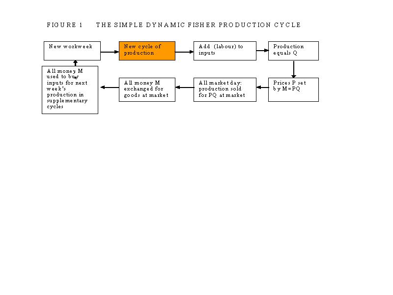
In practice, very little money
is needed if the speed of circulation V is high. In a very simple market
economy all the money could be exchanged every weekly market day. This is shown
in Figure 1.
Click here to view FIGURE 1 : THE SIMPLE DYNAMIC FISHER
PRODUCTION CYCLE.
Figure 1 is cash-based. In it, factors M, P and Q have been assumed
to be constant. The available money supply remains in circulation.
If, in Figure 1, PQ were greater
than M, not all of the goods for sale could be sold. Either M would have to be higher or P lower.
Over a year, the money M in
Figure 1 is circulated 52 times because there are 52 weekly markets, so V in
the Fisher Equation would be 52.
The V in the Fisher
equation refers to the speed of circulation of 100% of the money supply.
Humans are, by
nature, hoarders. Ever since money was first used, and especially after durable
metals like gold and silver were used for the money supply, people have “saved
for a rainy day.” The money physically
circulating at the market in Figure 1 was just a part of the total money
supply, not all of it. The rest was
“stored” 2. Instead of V in
the Fisher equation being 52 as shown in the simple example in Figure 1, it was
in fact much less because most of the money supply was hoarded. Despite that,
the value of V seems to have been more or less stable over long historical time
periods 3, suggesting the human tendency to hoard is psychological
as much as functional.4
3. Studies by the author
suggest that the speed of circulation V in
4. When the
amount hoarded is “enough” people will spend more.
Where the speed of
circulation V is constant it becomes more a structural than a dynamic component in the Fisher relationship. The immediate
response to a change in the money supply M will therefore tend to be a change
on the production side of the equation PQ.
If the change in M is rapid, the response will be a change in prices P
until production and demand adjust to compensate for the change in the money
supply. That’s different from what happens with fresh produce in the
supermarket after bad weather. In that case the money side of the equation
remains unchanged and prices rise because production falls. That happens in the
shops regularly and from season to season. Changing the speed of circulation V
would reflect either a change in people’s behaviour toward money, or changes in
the way the financial system works.
2.
DEBT AS MONEY.
Structural changes
in the money supply M began with the creation of new debt as money. When the Bank
of England was established in 1694, the money supply, for the first time,
became relatively independent of the supply of gold and silver.
When a bank issues
a new loan the loan becomes an asset in the accounts of the bank. The new loan
asset is offset by an equal bank liability in the form of a money deposit in
favour of the borrower. Money has been created “out of nothing” by way of a
bookkeeping entry. In the debt-based
financial system, for every dollar of money M there is a dollar of debt. Every loan must be repaid over time. As it is repaid, the outstanding loan is
reduced and the corresponding outstanding money deposit is also reduced by the
same amount. When the loan has been repaid both the loan and the debt have been cancelled out of existence.
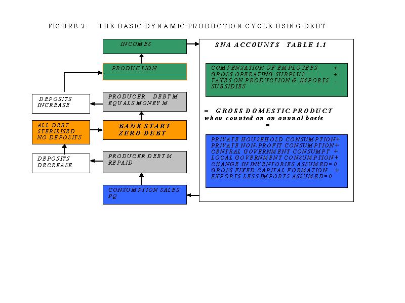
Unlike gold and
silver coins, debt cannot be hoarded. The debtor must repay the loan from
whatever deposits he or she can earn. That creates the production cycle shown
in Figure 2. For simplicity, the debt M
in Figure 2 is interest-free. Production and consumption are shown on the right
hand side of Figure
A fundamental
structural change has taken place. Whereas in Figure 1, the money M remains in
circulation, in the simple debt system shown in Figure 2 there is no money and
no debt left at the end of each cycle because each cycle is self-cancelling.
Click here to view FIGURE 2 :THE BASIC DYNAMIC
PRODUCTION CYCLE USING DEBT.
In aggregate, it is impossible
to save debt. It is, therefore, impossible to hoard or “save” money issued in
the form of debt in the debt system shown in Figure 2 without also increasing
debt. The cash component of a given money supply can, however, be hoarded. 5
In the real world,
production and consumption are going on all the time. There is always an amount
of debt M and its corresponding “money” deposits in use in the
dynamic economic
system. In this paper, the dynamic production
debt will be called My and its speed of circulation Vy.
Vy has
not been constant in the debt-based system because there have been structural
changes to the financial system itself. In industrialised societies, the role
of debt in the productive economy has increased over time. Cash transactions
now contribute very little to the measured GDP.
The proportion of employees paid weekly and the distribution of income
among employees, businesses and taxation shown in the upper right hand side of
Figure 2 have also changed 6.
There are also shorter-term variations. During recessions, business bill
payment time increases compared with the average while, during economic
expansions, it tends to decrease 7.
6. Indicatively
for
3.
INTEREST AND BANK SERVICES.
Interest has been
paid on loans ever since the use of money became widespread thousands of years
ago. People would loan their hoarded cash savings to someone else and expect
their savings to increase by the amount of interest they received. The borrowers would usually borrow in the
expectation that doing so would increase their productivity or their fortune in
some other way. For example, buying an ox or workhorse might dramatically
increase production from a farmer’s land.
The increased production created by using the ox or
the workhorse would more than offset the interest on the loan. Both parties
were better off as a result of the investment made by using the borrowed money.
The operative word
is “investment”. Investment is the use of money (originally cash, now mostly
debt) to increase production. The problem with the formation of the Bank of
England in 1694 was twofold. First, the
loans it made to the government of the day were not to increase production but
to help pay the war debts of the crown. Secondly the Ways and Means Act 8
that authorised the Bank of England provided for a perpetual fund of interest
charged on ships’ “tunnage” and liquor duties. Not only was the loan for
current spending instead of investment, it would never be repaid because the
Bank of England directors were happy to receive risk-free interest payments
forever. Since then, governments have found it very easy to borrow perpetual
debt in this way and its use has increased steadily over time.
The major change to the financial system brought by
the formation of the Bank of
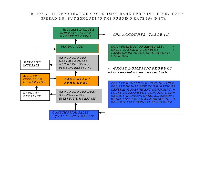
In the basic
dynamic cycle using interest-free production debt as shown in Figure 2, there
is no residual debt after any individual production cycle, and no residual
deposits.
The basic debt
system incorporating bank interest as part of the productive economy is shown
in Figure 3. There, the bank interest Is % is the bank spread 9. It does not include the funding interest If
% banks pay on deposits. Bank interest Is % is part of the
productive economy. Funding interest If % paid by banks on deposits
(net after tax) held by their clients is not productive.
8. 5 & 6
William and Mary C.20
9. The bank spread is the difference between the total loan interest (called the claims rate) and the interest the banks pay on deposits (called the funding rate). In this paper, bank spread is denoted by Is%, the bank funding rate by If % and the claims rate by Ic %, where Is%, = Ic - Ic .
Banks provide goods
and services just like any other business. Those goods and services are part of
the gross domestic product (GDP). The bank spread is a large part of the
“price” of banking. The only difference between Figure 2 and Figure 3 is that
in figure 3 bank services become part of Q in the Fisher equation output PQ and
the interest Is becomes part of the production debt My
already referred to on page 8. The production cycle is therefore still
self-cancelling as in Figure 2.
Click here to view FIGURE 3. THE PRODUCTION CYCLE USING BANK DEBT 10
INCLUDING BANK SPREAD IS%, BUT EXCLUDING THE FUNDING RATE IF%
(NET).
10. Figure 3 does not take
into account the effects of the current account.
The interest Is
banks charge to provide goods and services and the tax paid on funding interest
If is part of productive economic activity and does not cause
inflation.
4.
DEPOSIT INTEREST AND SYSTEMIC INFLATION.
Click here to view FIGURE 4 : THE DYNAMIC PRODUCTION CYCLE WITH DEPOSIT
INTEREST AND SYSTEMIC INFLATION SHOWING THE POOL OF RESIDUAL DEBT MSY WHERE
PRODUCTION Q IS ASSUMED CONSTANT.
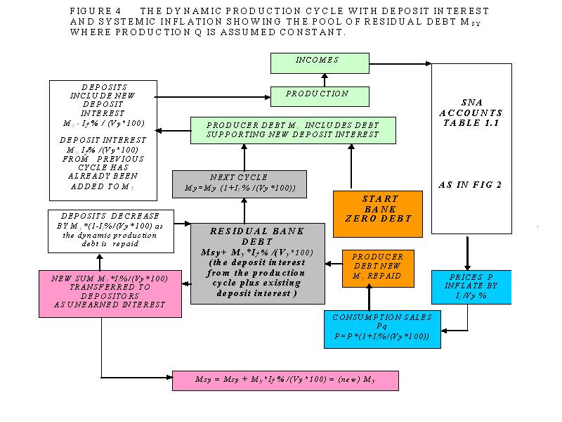
Figure 4 shows what
happens when funding interest If % is paid on bank deposits. The
dynamic production debt My is all repaid in full to the bank at the
end of each cycle. The funding interest If % paid by a bank is a
bank liability, not an asset. The deposits belong to deposit holders. The bank
must transfer to them the deposit interest it receives when the production debt
My is repaid. At first sight the bank would be losing money because
it would be left in debt by the same amount as the deposit interest.
In practice, the
production system does not “pulse” as shown for simplicity in Figure 4. Instead, there is an ongoing dynamic flow of
production and consumption funded by the dynamic production debt My.
The pool of residual debt (My in this paper) shown at the lower
centre of Figure 4 is the accumulated interest component My*If % /(Vy*100)
created through each nominal business cycle. 11 Since the
price P itself is the sum of the price increases shown at the bottom right of
Figure 4, price P must represent the total price inflation.
Assuming production
Q is constant, the deposit interest If
% (less tax) can be paid to depositors only if prices P increase as
shown. Otherwise the production debt My
cannot be cleared when the
economic production Pq 12 is sold. In this paper, the inflation
caused by the deposit interest on the dynamic production debt My is
called systemic inflation.
In an economy based on
interest bearing debt, almost all price is inflation.
11. My is a dynamic variable similar to those used in almost every iterative
computer program. The new total becomes the
old total for that variable plus the increment added to it each cycle.
12. The quantity
of production q is what is produced in the single nominal production cycle
shown in Figure 4. The amount q must be multiplied by the speed of circulation
Vy to get total output Q.
Click here to view FIGURE 5 : THE VISUAL CHALLENGE. CPI (CONSUMER PRICE
INDEX) ENGLAND 1300-2000.
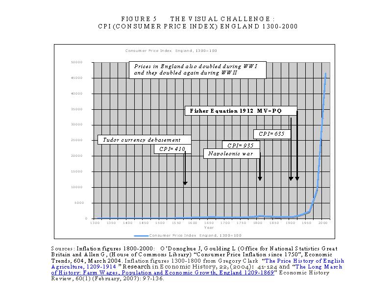
Figure 5 gives a historical
overview of inflation in
By the beginning of
the 20th century prices had increased by just 6 times in 600 years,
with nearly all the increases due to the “great debasement” of the mid-Tudor
period and the Napoleonic wars around the turn of the 19th century.
Prices fell by about one third between 1800 and 1900 during the industrial
revolution due to vast improvements in productivity. Higher productivity means more goods and
services are produced for the same input costs leading to lower prices P if
money M and speed of circulation V remain constant.
![]()
![]() The price change
formula P=P*(1+ If % /(Vy *100)) shown at the bottom
right of Figure 4 refers to a single production cycle producing the (constant)
economic output q. Figure 6 shows that, assuming the deposit interest rate If
and output Q are more or less constant, physical inflation is half of If
%. The figure P* If % /(Vy *100) is the rate of change of
P. It must be mathematically integrated to give the total change in P. This
increase in price in called systemic inflation.
The price change
formula P=P*(1+ If % /(Vy *100)) shown at the bottom
right of Figure 4 refers to a single production cycle producing the (constant)
economic output q. Figure 6 shows that, assuming the deposit interest rate If
and output Q are more or less constant, physical inflation is half of If
%. The figure P* If % /(Vy *100) is the rate of change of
P. It must be mathematically integrated to give the total change in P. This
increase in price in called systemic inflation.
Click here to view FIGURE 6 : SYSTEMIC INFLATION.
Systemic inflation
is a structural part of the debt-based financial system whenever interest is
paid on deposits.
Figure 7 compares
systemic inflation with consumer price inflation (CPI) in
Click here to view FIGURE 7. SYSTEMIC INFLATION
AND CPI INFLATION IN NEW ZEALAND..
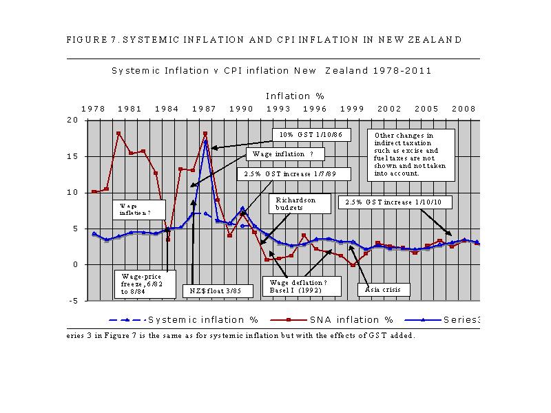
Rapid wage
increases increase the debt for production My faster than would
normally be the case. From the original Fisher Equation (1) MV=PQ, if M rises
while V and Q stay the same, P must rise in proportion to the rise in M. This is what happened before the debt-based financial
system became dominant after WWII as shown in Figure 5. It also seems to have
happened in
13. This raises
an interesting debate about comparing averages with indices and the
relationship between price indices and measured economic growth. The saw-tooth
form of the official SNA data in Figure 7 suggests serious issues with economic
management from 1978-1999.
14. The 1983 and
1985 years will still have been affected by wage factors even though they fell
partly within the period of the wage-price freeze.
When economic productivity
increases, more goods and services are produced using the same productive debt
My because, in aggregate, the unit cost of each item produced is a
little less than it was previously. In
the original Fisher equation
(MV=PQ), if M and V remain constant and Q increases then
P must decrease.
The price of many
items has fallen dramatically over the years as shown, for example, in Figure 5
during the industrial revolution in
Productivity growth
is inherently deflationary.
Labour productivity
is often measured by dividing the value of total production, the gross domestic
product (PQ), by the total number of paid hours worked. Capital productivity is often measured by
dividing PQ by the total current productive investment.. Education and skill
levels play a major in both measures because they allow new ideas and new
technologies to be introduced. Caution
needs to be used when applying productivity figures because the methods used to
measure them can be inaccurate. Typically, employees with higher education and
skill levels are paid more. That tends
to increase some incomes at the expense of others, distorting the income
distribution in most western economies.
The most extreme form of this is the very high compensation packages now
being paid to the executives of large corporations.
This paper assumes
that, in aggregate, wages inflate at systemic inflation plus the rate of productivity
growth to maintain overall price levels.
One key reason why so many employees in modern industrial economies feel
and are in fact worse off is because the benefits of productivity increases are
skewed as discussed above 15.
The increasing skew can be corrected only by income redistribution
within the economy.
15. Discussion of
the income skew is outside the scope of this paper, but one common way to
measure it is by using GINI coefficients.
The higher the coefficient the more skewed he income structure is. Over
the past 30 years
In a debt-based
economy where interest is paid on deposits, systemic inflation is half the
interest rate If paid on deposits provided adjusted incomes rise in
line with inflation and productivity growth and there are no changes to
indirect taxes.
Distributing the
benefits of productivity increases throughout the economy by improving real
wage levels and purchasing power requires socially mandated income redistribution.
Many developed
countries have failed to redistribute the benefits of increased productivity,
with consequent loss of consumption capacity in the wider economy. The classic
case of this in recent years is the tax cuts made by recent republican
presidents in the
Deposit interest
rates declined in
16.
17. Other possible
explanations are the backward “smoothing” of official data after the
introduction of the revised System of National Accounts (SNA93) in 1996 and the
implementation of the
5.
THE CURRENT ACCOUNT.
The current account
process is shown in Figure 8. The purple
box at the lower left shows how payments made on the current account in debtor
countries like
Click here to view FIGURE 8 : THE CURRENT ACCOUNT PROCESS.
18. The
Foreign ownership
of a debtor nation’s economy drains its domestic economic growth through
outgoing current account payments of interest on commercial paper and dividends
and profits arising from the physical foreign ownership of its assets.
Foreign ownership
of a debtor nation’s economy exposes it to high interest rates and the
permanent risk of capital flight.
In a debt-based
economy, it is not possible to both consume domestic production and pay for the
remittances to foreign countries covering interest and profit because that
would mean spending the same deposit twice. The cost of remittances for
interest and profit payable abroad must therefore be borrowed within the
domestic economy of the debtor country to enable the value of goods and services
produced there to be consumed.
The surplus goods
and services produced in a creditor country are part of its gross domestic
product and are counted towards its economic growth. When they are exported, so is the
growth.
A positive balance
on external trade exports domestic growth in exchange for foreign assets.
The deposits from
the sale of capital goods by a debtor country do not return to those who
borrowed the debt to pay for the surplus goods and services and remittances
sent offshore. They finish up, instead,
in the hands of those in the debtor country that have sold assets (or an
indirect claim on those assets) to settle the current account deficit. This means the debtor country’s capital
account must be reduced accordingly.
Contrary to popular
opinion, the direct borrowing of foreign currency by debtor country banks does
not increase asset inflation in the debtor country. This is because the
creation of the additional domestic debt used to fund the current account
deficit precedes the banks’ offshore borrowing. The bank “borrowing”
the foreign exchange simply “avoids” creating some of the deposits that would
otherwise result in the direct sale of assets in the debtor country to settle
its current account imbalance. If the creditor country banks chose not to lend
their foreign currency to the debtor country, the additional domestic deposits
that would necessarily arise from the sale of an equal amount of assets to
foreigners would further inflate domestic asset values in the debtor country.
Many, if not most,
of the debtor country deposits arising from the foreign “investment” as shown
at the upper left of Figure 8 fail to qualify as productive investment as
defined under the international System of National Account (SNA). They cause,
however, additional structural inflation through the payment of deposit
interest on the extra deposits. In that indirect sense, current account
deficits are always inflationary in the debtor country. The amount of inflation
depends on the interest rate paid on deposits in the debtor country and the tax
rate on interest income there.
The main
determinant of the exchange rate is the opportunity cost of capital in the
debtor country. It has to be “worthwhile for the creditor to “invest” in the
debtor country. When there is a free capital market the debtor must “match”
other investment options around the world. Otherwise the debtor country’s
exchange rate would need to fall until the investment prospect becomes “good”
enough for the creditor to “invest”. The base-line opportunity cost of capital
is the long-term bond rate in the debtor country. because bonds can be freely
traded. Almost the only determinant of the bond rate is the deposit interest rate
that must take foreign assessments of lending risk into account.
The main component
of the current account deficit in debtor countries is by interest paid on the existing accumulated current account
deficit.
At any point of
time, the current account deficit in heavily indebted debtor countries is
approximately the sum of the accumulated current account deficit x the average
bond rate - the trade balance for the preceding period + the net profits of
foreign-owned banks for the preceding period.
6.
SAVING AND INVESTMENT.
The use of the term
“saving” to describe a current account surplus is misleading. A creditor
country uses the surplus deposits on its current account to buy foreign assets
not because it has saved but because it has sold surplus production offshore
and received remittances from offshore. It is a trading dynamic, not a
conscious decision to forgo or defer consumption. It can be more a function of
overproduction than under-consumption.
The assets the creditor country buys mostly represent existing wealth
like equities, businesses, property, and related loans, rather than new
investment in bonds and business expansion in the debtor country that would be
defined as productive investment in the SNA. They are not “saving” as defined
in orthodox economic theory because most purchased foreign assets do not relate
to new domestic production in the creditor country and do not alter its gross
domestic product.
The purchase of
offshore assets and the provision of loans to offshore banks is, from the point
of view of the creditor country, income earning and “productive” at the price
paid for them, otherwise the exchange would not take place. That “income” is
not national income for the creditor
country because it cannot be remitted there. It forms part of the creditor
country’s current account surplus that is, in turn, swapped for more foreign
assets, and so on as long as the current account surplus continues.
From the debtor
country’s point of view, deposits arising from foreign capital inflows on the current
account qualify as “saving” in the debtor country national accounts only when they
are committed to new productive capacity. In reality, most capital inflows that
appear as domestic deposits in the debtor country represent “investment” in the
unproductive investment sector that serves to inflate the value of existing
assets or “wealth” there. That
“investment” neither adds to nor reduces production capacity in the
debtor country. It does not qualify as
investment under the System of National Accounts (SNA) and is therefore not
“saving” as defined in orthodox economic theory. Any deposits from the capital
inflows used to retire existing debt in the debtor country reduce debt and
deposits by the same amount. They do not affect the domestic economy of the
debtor country other than to reduce the systemic inflation caused by interest
payments on the domestic deposits a little.
Taking the current
account balance (CA) in creditor countries and debtor countries in turn the
sequence of the exchange that takes place is:
Any gross fixed
capital formation from return capital flows invested by a creditor country as
foreign direct investment in new capital goods in the debtor country is
automatically included in the GDP of the debtor country 19. The increase in the total
capital value in the creditor country contributed by the capital goods it
receives in payment of the debtor country’s CA deficit should be recorded in
its capital account. If it is to be treated as income, it must also be shown in
the creditor country’s income and outlay account.
In a debtor
country, gross fixed capital formation arising from any return capital flows
invested by the creditor country in new capital goods in the debtor country is
automatically included in the GDP of the debtor country 20. The decrease in the total capital value of
capital goods in the debtor country resulting from its sale of capital goods to
the creditor country in payment of the debtor country’s CA deficit should be
recorded in its capital account. If it is to be treated as negative income, it
must also be shown in the debtor country’s National income and outlay account.
19. It is assumed
that, since the debt that gives rise to the sale of capital goods in the debtor
country already exists, the deposits created from that debt also exist at any
point in time. Any productive investment arising from those deposits returned
to the debtor country in payment for its capital assets is therefore automatically
included in the debtor country’s domestic gross fixed capital formation.
20. It is assumed
that, since the debt that gives rise to the sale of capital goods in the debtor
country already exists, the deposits created from that debt also exist at any
point in time. Any productive investment arising from those deposits returned
to the debtor country in payment for its capital assets is therefore
automatically included in the debtor country’s domestic gross fixed capital
formation.
When the current
account balance is included as income in the national income and outlay account
of the SNA an entry of equal value entitled “purchase of capital assets on the
current account” should be included on the “use of income” side of the national
income and outlay account.
The National income
and outlay account of the SNA needs to be restructured to reflect orthodox
economic theory as follows:
Use of income side:
= Final
consumption C
+ Purchase
abroad of non-productive capital investment goods (=CA)
+ Saving for productive investment S. (2)
Income side:
= GDP
+ Current account balance (CA)
less the balance on external
goods and services
less repayments of principal
on outstanding productive investment. (3)
The National capital account
of the SNA needs to be restructured.
There is no “saving” residual on the “use of
income” side of the National income and outlay account because the items
“Purchase abroad of non-productive capital investment goods (=CA)” and the Current Account
Balance (CA) in equations (2) and (3) cancel each other out.
When Saving is
calculated as gross capital formation less principal repayments as shown in
equations (2) and (3) and used in Figure
Click
here to view FIGURE 9 : DISPOSABLE INCOME SHOWN IN THE NATIONAL
ACCOUNTS COMPARED WITH DISPOSABLE INCOME USING THE REVISED FORMAT NEW ZEALAND
1962-2010 21.
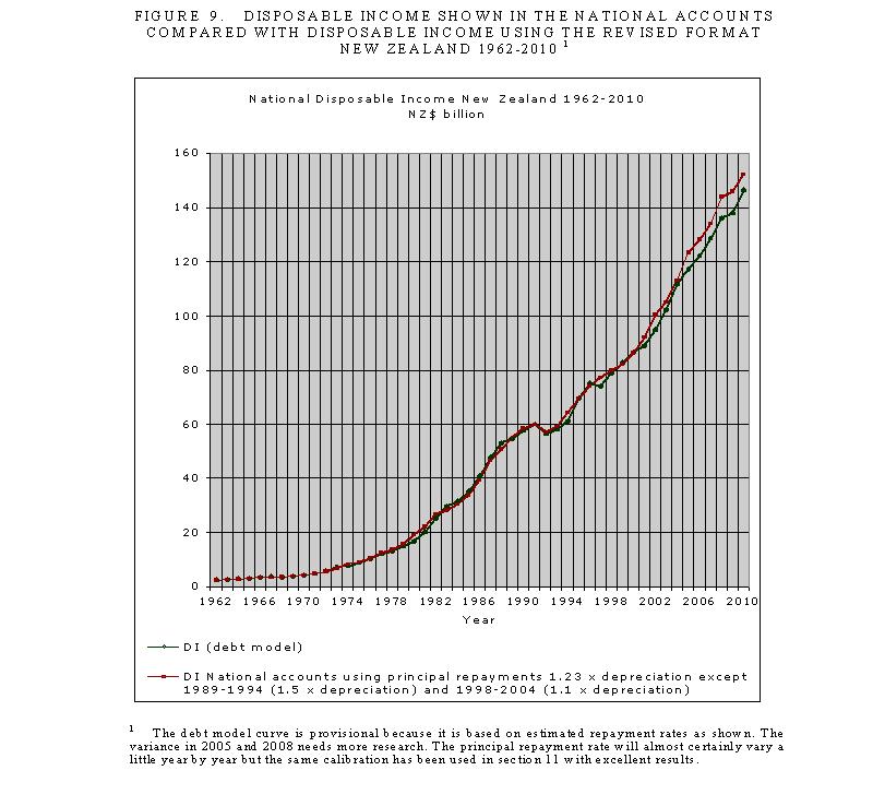
Click here to view FIGURE 10. NATIONAL SAVING S, AND NATIONAL SAVING S AS A PERCENTAGE OF
GDP* NEW ZEALAND 1962-1010. The GDP used in Figure 10 is
GDP as presented in the national accounts. Saving is gross capital formation
less the principal repayments calibrated as in Figure 9.
Saving in developed
countries, particularly debtor countries like
While higher
depreciation may in part reflect technological innovation and “planned
obsolescence”, its main effect has been to increase the ratio of principal
repayments to productive investment.
Higher repayment rates lead to a lower net operating surplus after debt
servicing and therefore a lower saving rate 23.
21. For example,
if the depreciation rate on a purchase of $10000 is increased from 20% to 25%
(therefore repaid in about 3 years) the extra depreciation is $500/year,
whereas the interest saved (at 10%) is just 10% of, say, a $650 extra annual
repayment, or $65 per year for 3 years; about $200 altogether. The firm’s
profit increases by roughly $300/year.
22.
United Nations, 2008 par. A.3.88 p.589 states: “The 2008 SNA
recommends that the consumption of fixed
capital should be measured at the average prices of the period with respect to a constant-quality
price index of the asset concerned”.
This appears to exaggerate the “depreciation “ effect on saving.
23. The debt
model curve is provisional because it is based on estimated repayment rates as
shown. The variance in 2005 and 2008 needs more research. The principal
repayment rate will almost certainly vary a little year by year but the same
calibration has been used in section 11 with excellent results.
Until now, there has been
little or no mention in economics literature of this structural impact on
saving.
National saving has been swapped for
short-term business profit, typically boosting stock and existing property
prices instead of longer-term investment.
Increased depreciation
allowances speed up principal repayments and reduce Saving S and Investment I.
7.
CREATION OF AND PAYMENT FOR CAPITAL GOODS.
Click here to view FIGURE 11 : INVESTMENT AND CAPITAL FORMATION.
Figure 11 shows how
capital goods are created and funded.
The basic economy without capital goods is shown in blue. The funding of
capital goods and subsequent repayments are shown in orange. The fundamental
orthodox investment equation (Savings= Investment) is shown in red.
The production of
goods and services giving rise to new capital goods is included in the
productive debt shown as My in Figure 11 24. Those new capital goods must be sold to clear
the market. Since the income earners in the productive sector who want to buy
the capital goods are not usually the same as those who produce the capital
goods, they are exchanged through bank intermediation.
24. See The interest-bearing debt system and its economic impacts for details of the debt model. The model is in
the process of being modified to separate the dynamic production debt My
physically needed to produce the GDP from the productive debt Mcd as defined in
the referenced paper.
The buyers of the
capital goods borrow part of the production incomes of employees (employee
incomes) and businesses (gross operating surplus) Sy=S/Vy where Vy is the speed of
circulation of Mv, as shown in the upper part of Figure 11. That
enables the original producer loans My to be retired, thereby
clearing the market.
In aggregate, some
employees and businesses have notionally swapped their share of the sale price
of the capital goods that they do not want to consume with others in the
productive sector (the investors shown
at the lower left of Figure 11) that do want to consume them. This creates
lending within the productive sector. There is a debt created in favour
of the “savers” in return for their deposit. After using the “savers’” deposits
to repay the production debt the investor has a debt as a liability and a
capital good as an asset, while the “savers” have an interest-bearing loan to
the investor as an asset to replace the deposit they had in the bank.
Whatever bank
intermediation takes place, in aggregate, the process shown in Figure 11 must always be true if the goods and services
Q produced by the productive sector are all to be sold to clear the market.
Where that does not happen, there will be consequential changes in
inventory.
The main feature of
the exchange discussed above is that the investor debt is interest-bearing and
accumulates with each production cycle.
The investment and
capital formation shown in Figure 11 is dynamic. The faster the rate at which
investors repay their debt, the less Saving there will be, because Saving = New
investment less repayment of outstanding capital.
Increased repayment
of debt, including household debt, reduces Saving and reduces net new
productive Investment.
Any attempt to withdraw
any part of deposits S/Vy for
non-productive investment purposes (“savings”) reduces purchasing power in the
productive economy or leaves capital goods unsold, leading to increases in inventory, and
subsequent unemployment and recession.
In
“Savings” schemes
such as Kiwisaver in
It is impossible to
increase GDP or Saving without increasing production loans My and
new productive investment.
Increases in
inventory, other than what is needed to allow for inflation and population
growth, have very little, if any, value despite their being entered in the
National Accounts as “investment” at cost.
Added inventory and subsequent production must later be discounted to
clear the build-up, otherwise inventory would continue to grow.
There is always an outstanding production debt My
that is continually being recycled through the production system and there is
always a corresponding flow of Saving Sy = S/Vy and
investment Iy = I/Vy for the production of capital goods.
Economic policy planning and implementation must
be based on a progressive dynamic supply of new productive debt My
to make use of spare labour and resources in the economy or to increase the
skills of, and re-employ existing resources.
Capital formation takes place by new debt
formation within the productive sector itself and domestic productive
investment in terms of the SNA can be viewed as the redistribution of
production incomes to clear the capital goods market in the productive sector.
Capital formation as it is shown in Figure 11 of this
paper follows the basic tenet of orthodox economics that Savings=Productive
Investment.
Investment in new residential housing consumes
part of the Savings Sy=S/Vy
in Figure 11. As noted at the lower right of Figure 11, most housing investment
is, however, economically unproductive once it has been built. Furthermore,
the more new housing investment there is, the less is available from Sy
for other productive investment. Assume, for example, that in
Not only does housing construction slow the
growth of economic consumption, it is very difficult for the buyers of new
homes to repay their mortgage debt without decreasing their own existing
consumption. As shown in Figure 4, incomes nominally increase at only the rate
of systemic inflation. As discussed in section 4, systemic inflation is half
the deposit interest rate. The increased income of homeowners is therefore not
enough to repay the interest on their mortgages, let alone repay any principal. It follows that to own their new homes
homeowners must consume less by an amount equal to their principal repayments
plus their mortgage interest.
In the absence of productivity gains, new
homeowners must reduce their domestic consumption by an amount equal to
principal repayments plus their interest cost.
In the distant past, the income deficit could
have been met by large labour productivity gains. Increasing labour
productivity is deflationary because, unless extra incomes are injected into
the economy to cover the purchase of the extra production, it makes available
more goods and services for the same production cost.
Consumption could be maintained as long as the
productivity increase was enough to offset, in aggregate, the additional
interest and principal payments being made by households
25. Suppose for example,
outstanding home mortgage debt is $100b and GDP is $200b and that interest
rates are 7%, bank spread 2% and principle repayments 3%. The total productivity increase would need to
be 7% + 3% or 10% x S100 b = S10 b. $10b/200b = 5% of GDP. Productivity increases like that do not occur
in developed economies because developed economies are largely service-based.
Allowing 1% for productivity increases means a deficit of 4% of GDP before
taking into account population changes and changes in the balance of trade.
More recently, indebted homeowners have instead been
working longer hours, often by switching from single-income households to
two-income households. While indebted households may manage to keep up their
mortgage payments by working longer and/or with two members working instead of
one, there is a corresponding structural decrease in consumer demand that
cannot be satisfied within the productive economy. That structural decrease in
consumer demand is the result of interest and capital payments homeowners must
make to repay their household debt. Either consumers in aggregate must be
induced to borrow outside of the productive economy to maintain demand (for
example, by re-mortgaging their homes) or there will be growing structural
unemployment as production is reduced because of the oversupply of consumption
goods and services. The only other option is to export the surplus consumption
goods and services.
In practice there is a combination of outcomes
with some productivity increase, perhaps 1% annually in New Zealand, developing
structural unemployment and some (extra) consumer debt to temporarily maintain
demand. There should also be an improvement in the balance of trade. Additional
debt can be generated using house price inflation as the security for new
loans. However, the additional consumer
debt cannot be repaid out of existing incomes any more than the indebted
homeowners can repay their loans from their incomes. In both cases the extra
debt makes the productive economy worse and not better off in the longer term
due to falling consumption capacity. The classic result of this was the
sub-prime crisis in the
In the long run, homeowners cannot repay their
mortgage debt without causing increasing structural unemployment in the
productive economy. They can export the surplus consumption goods and services
they cannot themselves consume This will alter the balance of foreign ownership
of the domestic economy but not the wellbeing of its people.
Residential housing
investment that does not generate income is fundamentally incompatible with a
financial system based on interest-bearing debt.
SECTION
8. THE DEBT MODEL.
The first version
of the debt model was published in the paper:
Manning, L “The Ripple Starts Here: 1694-2009 : Finishing the
Past”, presented at the 50th
Conference of the New Zealand Association of Economists (NZAE),
While the debt
model is based on the volume of debt, it is unrelated to earlier volume-based
reform proposals like those of Social Credit that failed to offer a viable
theoretical basis to support them.
The premise in both
the debt model and Figure 4 is that the circulating deposits and cash My
= Prices P x output q where q is the quantum of domestic output produced by My
over a single cycle. Taken over a whole
year, the SNA definition of Gross Domestic Product GDP is given in the debt
model by mathematically integrating the expression Pq* Vy, where Vy
is the number of times the circulating deposits and cash My are used
during the year 27.
The SNA should
reflect an expression of the original Fisher Equation of Exchange as shown in
Figure 2 28. The only
difference is that the money supply M in the Fisher equation of exchange included
hoarded cash, whereas in the debt system shown in Figure 2 for practical
purposes there is now very little cash contributing to measured GDP.
In Figure 4 My
cannot include hoarding of debt beyond the term of the production cycle because
all the productive bank debt giving rise to My is conceptually
repaid at the end of the cycle 29.
26. http://www.nzae.org.nz/conferences/2009/pdfs/The_Ripple_starts_here_1694-2009__Finishing_the_Past.pdf
. Non-members can access the paper by Google search: NZAE The Ripple Starts
Here (use “quick view”).
27. The
contribution of cash transactions in industrialised countries is now (very) small.
28. The Fisher
equation has been very widely discussed in relation to the economic
difficulties arising from the sub-prime mortgage defaults in the
29. As previously
noted, in practice there is a continuous flow of production and consumption so
the deposits and cash My are always
present, but they are being used in the production cycle, not hoarded.
At any point in
time there are five broad blocks of deposits in the domestic financial system.
They are:
Mt The transaction deposits representing the
productive debt My - M0y so:
My
= Mt + M0y (4)
Mca The
accumulated domestic deposits representing the sale of assets to pay for the
accumulated current account deficit (see section 5 of this paper for
details).
M0y The cash in
circulation included in Mv and used to contribute to productive
output.
Ms The net after
tax accumulated deposits arising from unearned deposit income on the total
domestic banking system deposits M3 (excluding repos) 30.
(M0-M0y) Cash hoarded by the public and not used
to generate measured GDP.
In this paper the
total of these deposits, that is, Mt + Mca + M0y
+ Ms , is provisionally assumed to be the M3 (excluding repos)
monetary aggregate published by most central banks monthly less the amount of
cash in circulation M0 except for the part M0v that is included in My. In this paper M0y is assumed to
have the same speed of circulation as My. In industrialised countries, the contribution
of cash transactions to the measured output of goods and services (GDP) has
been declining in recent decades and their contribution to the GDP has been
provisionally calibrated for the purposes of this paper 31.
In this paper, the
total debt in the domestic financial system is assumed to be the Domestic
Credit, DC debt aggregate published by most central banks monthly.
At any point in
time there are four broad blocks of domestic debt in the domestic financial
system. Three of them together add up to DC such that:
DC = Dt + Dca 32 + Ds
(5)
Where
Dt The
productive debt supporting the transaction deposits Mt.
Dca The whole of the debt created in the
domestic banking system to satisfy the accumulated current account deficit 33.
Ds The residual debt to balance equation (5)
30. Repos refer
to inter-institutional lending
31. More accurate
assessment of the cash contribution to GDP over time requires further detailed
study.
32. Arguably the
accumulated sum of capital transfers could be included here, in which case the
net international investment position (NIIP) would be used instead of the
accumulated current account. The decision affects the size of the “residual” Db.
33. This is
greater than the monetary deposits Mca because the
banking system may have sold commercial paper to borrow foreign currency to
satisfy the foreign exchange settlement as shown in Figure 8.
The fourth block of debt is :
Db, the virtual “bubble” debt, the excess
credit expansion or contraction in the banking system such that Ds - Db = the debt supporting the accumulated deposit interest Ms defined
above. Db can be positive or
negative as discussed further below in relation to Figure 5.
There is also a
fifth block of debt Is that is, conceptually, not bank debt .
Is, the
total debt accumulated by investors arising from Saving Sy = S/Vy.
In Figure 11, the
investor pays the investment Iy =I/Vy = Sy =
S/Vy to the producer and the
money is used to retire the outstanding part of My relating to the
investment in question. Conceptually the investor borrows the purchase price
from employee incomes and the business operating surplus as discussed in
section 7. Except for households buying new homes discussed separately on pages
27-28, the investor then becomes a producer, and the interest on investment Iy
is included as a production cost in the subsequent production cycle loans My.
The predicament of
new homeowners is quite different. They cannot service their debt because they
cannot, conceptually earn more than they were before they bought their new
home, because the home itself is nearly always unproductive. There is no new
income stream from their housing investment. If economic demand is to be
maintained, homeowners must, in aggregate, rely upon increasing house prices
and refinancing of their properties, creating an aggregate “pass the baton”
systemic increase in debt.
When non-productive investment assets are
traded there is typically a capital gain because of asset inflation on
investment (Dca + Ms + the property component of Is). The new purchaser pays more for the asset
because of asset inflation, allowing the seller to retire the outstanding
mortgage debt on the property.
By definition in this paper :
My x Vy
= GDP
Ms = Ds
The cash contribution to GDP =
M0y * Vy. Therefore :
DC = (GDP)/Vy - M0y + Ms + Dca
+ Db (6)
Ms =Ds =
(DC – Dca ) – GDP/Vy + M0y - Db (7)
GDP = Vy *(DC - (Ms +Dca
+Db ) + M0y ) (8)
My = GDP/Vy
= DC - (Ms +Dca + Db) + M0y (9)
Where the terms are as defined
on pages 28-29.
Equations (6 ) to
(9) are all forms of the debt model developed in previous papers 34.
34. Links
are provided in the conclusion to this paper.
Ms is
the same format as Ms in the earlier forms of the model. It has been freshly
calibrated. Unlike the previous forms of the model equations (6) to (9) are
general and include the contribution made to the economy by cash transactions.
In equation (7),
all the terms except GDP/Vy = My and Db are
known or can be estimated with reasonable accuracy. For the purposes of
equations (8) and (9) My can
be approximated using trend-lines because it is small compared with Ms.
Db is unknown but can be approximated through the calibration as in
Figure 5. The calculations in equations (8) and (9) involve the subtraction of
large numbers to get relatively small numbers, which leaves them sensitive to
modelling and data error.
If Ms,
calculated as “the accumulated deposits arising from unearned deposit income on
the total domestic banking system deposits M3(excluding repos) ” as
defined on page 30, agrees more or less with that calculated in equation (7),
bearing in mind the value of Mb, the proposition that debt growth is
determined by deposit interest will be proven.
The model will require further calibration as further data becomes
available. Despite that, it is
self-evident Db will be positive during periods of rapid expansion,
particularly as bubbles form, and will become negative during periods of rapid
contraction, particularly as bubbles collapse. The classic case of this in
The dependence of
the gross domestic product (GDP) on the Domestic Credit DC and the interest
rate on bank deposits in the modern cash-free economy from which Ms
is calculated has profound implications for economics.
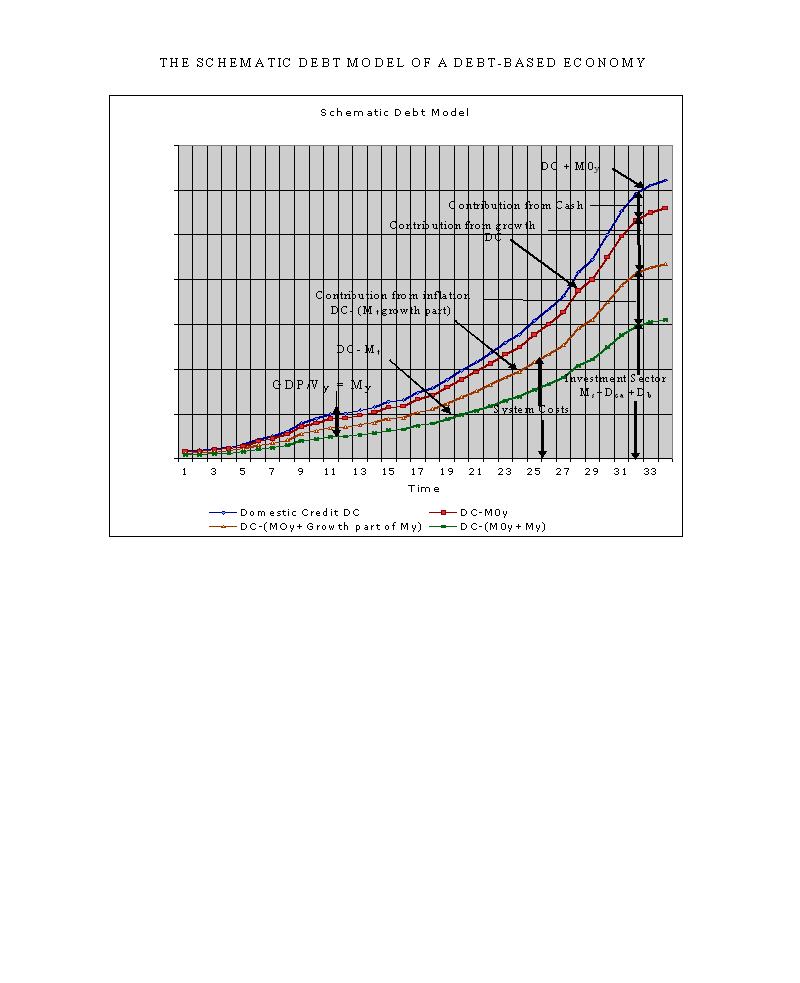
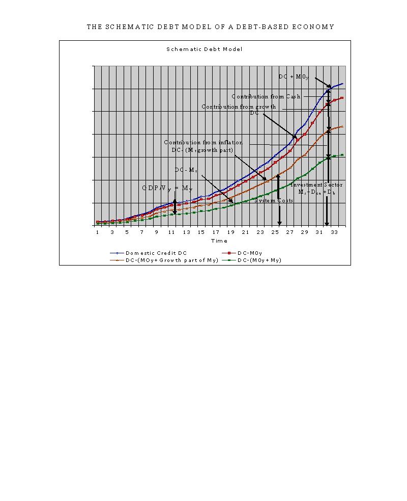
In the light of the
worldwide financial chaos of 2007-2009 the indicative debt model shown in
Figure 12 provides a powerful argument in support of public control of a
nation’s financial system.
Click here to view FIGURE 12 : THE SCHEMATIC DEBT MODEL OF A DEBT-BASED ECONOMY.
The vertical axis
in Figure 12 applies to the Domestic Credit for
It isn’t possible
to have a simpler model of the economy than equation (8):
My
=Nominal GDP/Vy equals domestic credit DC less (unearned net deposit
income Ms + the accumulated current account Dca + the
cash contribution to GDP M0y plus a correction for bubble activity Db
(+/-))
Domestic
Click here to view FIGURE 13 : EXPONENTIAL DEBT AND
GDP NEW ZEALAND, 1993-2011.
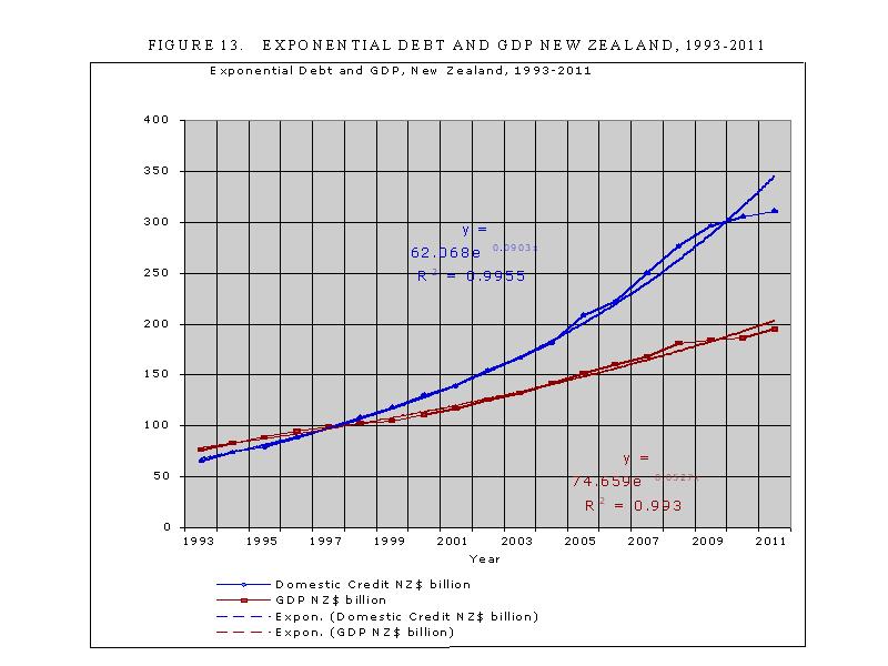
It is theoretically impossible
to maintain exponential debt expansion faster than GDP expansion over an
extended period because the added debt servicing costs will always leave the
productive sector insolvent.
To avoid national
bankruptcy, each nation must maintain, in aggregate, a zero accumulated current
account deficit.
A first
approximation for the speed of circulation Vy of productive debt
plus cash transactions My is given in Figure 14. Vy varies with the change in the
payments systems. Minor secondary shorter-term cyclical variability also occurs
through changes in the average time taken to pay bills. When times are tough people take longer to
pay their bills, and each change of a day in the time taken to pay them can
alter Vy by perhaps 0.25%. The process is usually reversed in better
times. Otherwise Vy reached a constant value of about
35. Vy is estimated at the moment so the present figures are indicative. Once
further research accurately refines the present estimates, Vy will be sufficiently accurate for predictive purposes.
Click here to view FIGURE 14 : SPEED OF CIRCULATION Vy NEW ZEALAND 1978-2011.
Note that in Figure
14, no correction has been applied to Vy for secondary increases in
payment time during recessions or decreases in payment time during economic
boom periods. The maximum correction in Vy appears to be in the
order of +/- 0.3 or up to 1.5%. The series shown is less stable from 1978 to
1989. This is possibly due to distinctly different growth exponentials
1978-1989 arising from the very high interest rates that were typical during
those years.
As shown in Figure 15, My in
Click here to view FIGURE 15 : ESTIMATED TRANSACTION FUNDING My NEW ZEALAND 1990-2011.
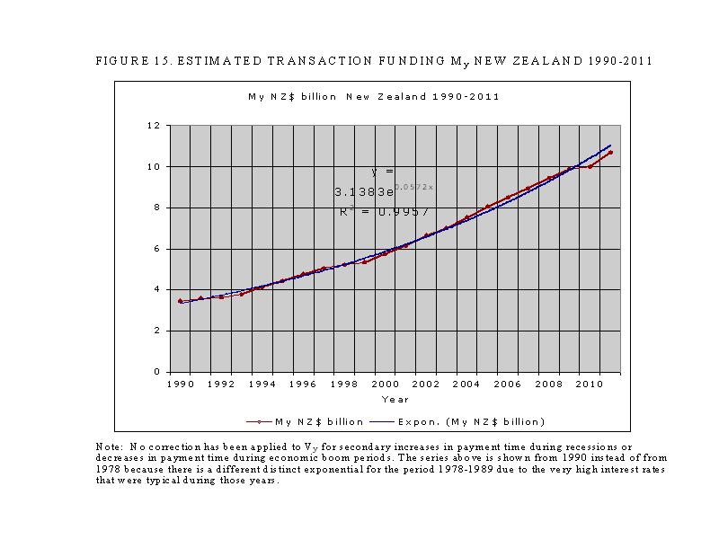
The methodology
used to calculate Vy in Figure 15 is as follows. The GDP in
Businesses pay
suppliers monthly, and indirect payments are usually made on a monthly basis
too, so their speed of circulation is about 12 on average. Most workers get
paid fortnightly (though some get paid weekly and some monthly) so an average
speed of circulation of 26 has been assumed for that.
When the above figures are
weighted the weighted average speed of circulation is (12x(42.7+12.3)+45 x
26)/100 = 18.3.
A similar estimate
of payment trends and a separate Vy calculation was made for each of
the other years, and a polynomial best fit curve was drawn as in Figure
15.
My was
then obtained by dividing the official GDP figure by the speed of circulation
taken off the best fit trend curve. This
gives the data series shown in Figure 16 and used when applying the debt model discussed in
section 8.
The methodology is
easily replicable using better information about payment trends and is
applicable to any country.
Figure 15 shows the
preliminary estimate for estimated production debt and cash My in
Figure 16 shows an
indicative comparison between the residual debt Ds for New Zealand
calculated from equation (5) and plotted against the model Ms
calculated as the accumulated after tax deposit interest on M3 (excluding
repos). The curve for Ms is a first approximation because
assumptions have been made on the average tax deducted from the gross payments
of unearned income (M3 (excluding repos x the average interest paid on
deposits). The tax is the average tax
paid by each income-earner on his or her total income. It is not the marginal
tax rate 36. The losses from
the 1987 share market crash in
Once the tax rates
on Ms have been accurately calibrated, the size of any debt bubble Db
can be immediately calculated.
Measures can then be taken to eliminate the bubble without risking any economic
downturn.
Click here to view FIGURE 16 : BUBBLE DEBT Db AND Ms NEW ZEALAND
1978-2011.
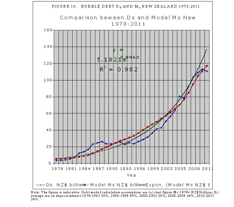
9. DIFFERENTIAL ANALYSIS DEPRESSIONS AND
RECESSIONS.
Equations (6) to
(9) can equally be applied in their differential form by calculating
differences from one period to the next.
For example, over
any small period of time dt, the change in the total debt DC = the change over
the same time dt of ( GDP/Vy - M0y + Ms + Dca + Db ).
There is quite a
lot more variability in the figures calculated this way compared with equations
(6) to (9) because
additional error is introduced by multiple subtractions of large numbers.
Using the
differential approach (and Newtonian notation) allows the new debt model to
show how the economy is performing in practice. With better data economic performance
could be assessed monthly, or even, theoretically, in real time. The
differential equations are:
d/dt DC = d/dt ( GDP/Vy - M0y
+ Ms + Dca +
Db )
(10)
d/dt Ms =d/dt Ds
= d/dt ((DC – Dca ) – GDP/Vy + M0y - Db ) (11)
d/dt GDP = d/dt (Vy *(DC
- (Ms +Dca + Db ) + M0y
)) (12)
d/dt My = d/dt GDP/Vy = d/dt (DC - (Ms +Dca + Db) + M0y (13)
where:
DC = Domestic Credit debt aggregate published monthly by central
banks.
GDP = Gross Domestic Product
(the same as economic output PQ in the original Fisher Equation
Vy = The speed of circulation of the
productive debt My
My = The dynamic productive debt used to
generate output (see Figure s 3 and 4)
My is interchangeable
with GDP/Vy in equations (10) to (13).
M0y = The cash in circulation included in Mv
and used to contribute to productive output.
Mt =
The transaction deposits representing the productive debt My - M0y
so:
Ms = The
net after tax accumulated deposits arising from unearned deposit income on the total domestic banking system
deposits M3 (excluding repos) 37.
Dca = The whole of the debt created in the
domestic banking system to satisfy the accumulated current account deficit 38.
Ds = The
residual debt to balance equation (5)
Db =The virtual “bubble” debt, the excess credit
expansion or contraction in the banking system such that Ds - Db = the debt supporting the accumulated deposit
interest Ms.
37.
Repos refer to inter-institutional lending
38. This is
greater than the monetary deposits Mca because the
banking system may have sold commercial paper to borrow foreign currency to
satisfy the foreign exchange settlement as shown in Figure 8.
For example, in
d/dt DC =
d/dt (GDP/Vy - M0y
+ Ms + Dca + Db) (10)
NZ$ 26.4b
= 0.73 + 0.02 + 10.01 + 13.34 +
d/dtDb
=
NZ$24.1b + d/dtDb .
This shows the credit bubble
grew by about NZ$ 2.3b in the March 2008 year.
Figure 16 shows the
bubble surplus Db growing in the March 2008 year (upward slope of Ds
relative to Ms), accounting for the difference between the official
figure and the derived one. The example above is within the statistical error
of the official data even before taking Db into account. More
calibration work is needed before using the differential method for predictive
purposes, particularly in equation (12) that requires a small number to be
multiplied by Vy to get the change in GDP 39.
39. There are
periodically quite large revisions in the official statistical data, too, that
make all the national account data estimates rather than facts.
An approximate
check of the calibration is readily available because in Figure 16, Db
should be zero where the model Ms curve intersects the Ds
curve. Some obvious years to check are 1982, 1992, 2004 and 2009 though the two
curves do not cross exactly at the data points.
In Figure 16 using
the nearby data points the “error” between Ds and Ms in
1982 is -1.0% of GDP (Ds slightly larger than Ms). In
1992 the error is + 1.7%, in 2004 +1.4%, and in 2009 -1.8%. The error between
the Ds curve and the Ms curve is within acceptable limits
given the preliminary nature of the model calibration and the accuracy of the
official data series.
A non-zero figure
for Db in the debt model represents an imbalance between existing
debt and economic performance, and it indicates unsatisfactory financial
management.
When Db
in the debt model is negative a credit bubble exists and when Db is
positive an economic contraction is taking place. When the slope of the bubble
is rising (upwards over time) the bubble is intensifying and when it is falling
(downward over time) it is dissipating. The bubble is not fully dissipated
until the Ds curve meets the Ms trendline and Db
has returned to zero. When the slope of the recession is falling (downwards
over time) the recession is intensifying and when it is rising (upward over
time) the economy is in recovery. The recovery is not complete until the Ds
curve meets the Ms trendline and Db has returned to zero.
Figure 16 shows
that in
From equation (12), when d/dt
GDP = 0
d/dt GDP = d/dt (Vy *(DC
- (Ms +Dca + Db ) + M0y)) (13)
Since in a fully debt based
financial system M0y is zero and d/dt Db is usually small,
d/dt DC =
d/dt (Ms+Dca
) approximately (14)
In a debt-based
financial system, if there is no increase in the total economic output,
domestic credit must still increase by the amount of unearned income that has
to be transferred to the investment sector Ms plus any current
account deficit that has to added to Dca. Unless there is residual
bubble debt Db in the financial system, failure to maintain
sufficient domestic credit as in equation (14) would be accompanied by economic
collapse because GDP would necessarily fall by any shortfall in domestic credit
x Vy.
The provision of
new debt for inflation in the debt model together with unearned income and the
current account deficit can together be considered financial system costs.
Economic growth occurs only when and to the extent that d/dt DC exceeds the
financial system costs as shown in Figure 12.
A recession
provides for inflation but not economic growth, while a depression provides for
neither economic growth nor inflation.
A recession occurs
when the change in the total debt over time is less than what is needed to
service the financial system costs made up of the net unearned interest that
has to be paid on all bank deposits plus any new current account deficit plus
any increase in the productive debt used to generate new economic output. In
that case, d/dt DC is less than d/dt
(Ms+Dca ) plus provision for inflation.
A depression is a
deep recession. It occurs when the change in the total debt over time is less
than what is needed to service the unearned interest that has to be paid to the
accumulated net deposit interest Ms plus any current account deficit
that has to be added to the accumulated current account deficit Dca,
that is, when there is no provision for either inflation or growth.
The model can be
used to provide specific measurable monetary targets to avoid recessions and
depressions. The targets can easily be identified in advance and new debt
injected into the system to maintain growth limited only by the resources
available and the productive capacity, education and knowledge of employees and
businesses.
The amount of new
productive debt d/dt My needed to fully utilise the available
resources and the productive capacity, education and knowledge of employees and
businesses is very small. In
40. It may even be that all is needed is a public guarantee that any excess production during the recovery period will be purchased, in other words a state guarantee to give businesses the confidence to produce.
The collapse in the
capitalist system is caused, in part, by its failure to recognise that
production must, just by a little bit, lead consumption to provide the incomes
that enable consumption to take place.
In recent decades
it has been assumed that lower interest rates would be enough to restart a
stalled economy. That is no longer true. The exponential growth of debt required
by the debt-based system itself means that the increase in consumption
capacity generated by an interest rate cut is no longer sufficient to allow an
economy to recover.
For example, in
March 2011, domestic credit in
Interest rate
reductions only work to stimulate an economic recovery when asset inflation
remains high enough for the debt generated by refinancing and trading of
existing assets to offset the systemic debt requirements of the financial
system.
The logical outcome
of the existing debt system in creditor countries is zero deposit interest and
stable or falling asset prices (as in
In the absence of
strong capital controls, the logical outcome of the existing debt system in
debtor countries is bankruptcy because debtor countries must maintain high
rates of interest to avoid capital flight. The debtor status of debtor countries
can only be reduced if their exchange rates are reduced so their current
accounts become positive enough to reverse the foreign ownership of their
assets.
There is a powerful
theoretical incentive for public investment in new production to assist a
market economy out of recession or depression. That investment in the first
instance needs to be in new means of production to provide incomes and
employment to relieve the fiscal pressure on public social welfare expenditure.
Once the market economy fails, as it does in recession, it cannot recover
without a stimulus sufficient to encourage the private sector to invest and
produce. Until the private sector does so, the production cycle is effectively
broken.
Government has a
fundamental role to stimulate an economy when it enters a recession by directly
investing in new production.
Infrastructure investment is too slow to be useful because there is a
long lead-time before increased productivity exceeds the infrastructure costs.
10. EQUITY IN SOCIETY.
Figure 17 shows
compensation of employees plotted against the operating surplus for
Click here to view FIGURE 17 : COMPENSATION OF EMPLOYEES v GROSS OPERATING SURPLUS NEW
ZEALAND 1978-2009.
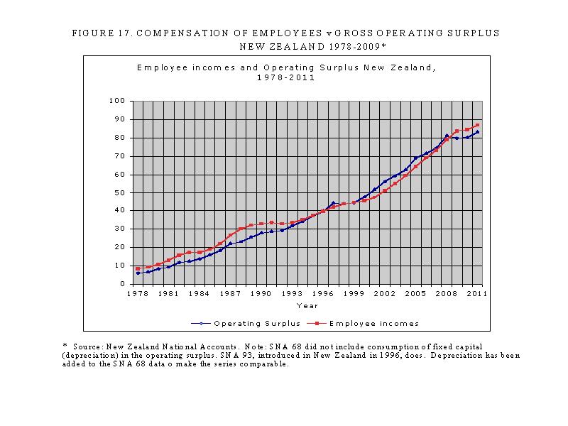
The System of
National Accounts (SNA) version 68 (1968) did not include consumption of fixed
capital (depreciation) in the operating surplus. Version SNA 93, introduced in
One common way of
measuring income equality is by using the Gini coefficient
Over recent decades,
Since 2007, the
Gini coefficient for
Poor income
distribution suppresses demand for domestically produced goods and services.
People with low incomes have relatively little to spend on domestic
consumption, especially on services, which make up the bulk of monetised
economic activity. Income concentration encourages relatively high demand for
imported “luxury” products adding to
41. It remains
possible the relationship between the numbers of entrepreneurs and the numbers
of wage and salary earners has altered, for example if firms became bigger on
average. Such changes would not be disclosed in Figure 17.
42. The Gini coefficient
is developed from the Lorenz curve, which is a plot of incomes against
population starting from the poorest groups in the population, There is a good
introduction at http://en.wikipedia.org/wiki/Gini_coefficient. The coefficient usually excludes investment
income.
43. The Gini
curve used for these figures was taken from the NZ Green Party website 19/6/10
because it is reasonably current. http://blog-greens.org.nz/2010/04/06/inequality-in-aotearoa-a-brief-history-of-inequality/ Various organizations like the UN and the CIA
calculate Gini coefficients which can vary depending on the way the basic data
is compiled.
44. This does not
suggest
There are just two
ways to avoid large earned income imbalances. The first way is to increase
lower end wages and salaries, especially minimum incomes. The second way is to
reconsider taxation policy, not for political reasons but because the existing
income distribution structure has not been working well. Both the debt model
referred to Section 8 of this paper and the analysis in Section 4 show that
inflation and growth must be reflected in incomes for the production cycle to
clear. Heavily skewed income distributions make the process of clearing the
market from each production cycle more difficult. Some people have “too much”
(and growing) income in relation to domestic consumption and many others “too
little” (and falling) income. “Ordinary” employment gets squeezed. That’s why
the economies of social democracies have tended to perform better than the more
capitalistic ones in recent times.
Every economy can
be thought of as having its own physical shape. That shape reflects the degree
of “reasonable self-sufficiency” the economy possesses. Reasonable
self-sufficiency describes how well domestic production matches the consumption
patterns of the population as a whole taking into account its income structure.
The less of its own domestic product an economy can afford to consume and the
more reliant that economy becomes on importing what it needs but does not
produce, the more skewed the economy becomes. The more skewed the economy the
more dependent it is likely to be on foreign trade, globalisation, and in some
cases, on the foreign ownership that arises from large accumulated current
account deficits.
Income distortions
have become structural, especially in industrialised capitalist economies.
According to the debt model, increased incomes are inflationary unless they are
accompanied by corresponding increases in productive output. Since the employed
workforce is already producing goods and services, the SHAPE of the economy,
the basket of goods and services produced in relation to incomes and
consumption patterns, will have to change if it is to improve the lot of the
people as a whole so that everyone gets a “fair” share 45. Increasing incomes without increasing
production would just increase prices.
Changing the shape
of the economy means eliminating excessive debt, especially the domestic
debt arising from current account deficits. It also suggests changing the tax
structure.
Tax structures in
most parts of the world are confusing, antiquated and expensive to run. They are layered like an onion. New taxes
have been added over the centuries as the means to collect them have become
available. They are full of loopholes and exceptions granted to vested
interests of one kind or the other. Governments of all hues have tended to
weight tax law with an eye towards their own perceived constituencies and
re-election. This implies short-term goals have been adopted instead of
policies for the long-term benefit of the nation as a whole. Governments claim
to know the importance of goals such as economic efficiency, research and
development, the “knowledge” economy, investment and the reduction of welfare
dependency but they are unable to “walk the talk”. Systemic constraints have
made effective political action to adapt the existing financial architecture to
the needs of modern economies all but impossible. The current financial system
has become a straightjacket on the world’s economies as the recent debt “crises”
have demonstrated, with
In
45. What that
“fair” share is should be a defining political debate in a democracy.
46. GST refers to Goods and Services Tax. In
The SHAPE of an
economy is largely determined by its income distribution.
Skewed tax systems
relatively benefit a small section of society at the expense of everyone else.
Skewed tax systems
impair economic performance and economic growth potential by systemically
transferring purchasing power from the productive sector to the unproductive
sector through increased debt and debt servicing.
A flat tax to
achieve tax universality is available to governments that choose to use
it. It is called a Financial
Transactions Tax (FTT) 47. FTT is very cheap to run. It could easily
replace all other forms of taxation except social excise and environmental
taxes such as those on tobacco, alcohol, fuel, pollutants, and perhaps source
deductions on sugars and saturated fats that contribute heavily to obesity,
diabetes 48 and heart disease. Most of the nations’ Revenue
Departments could be dismantled. One version of FTT is to deduct the tax
automatically every time money is transferred out of any deposit account unless
the transfer is to another account held by the same account holder. Savings in
downstream compliance costs (government, accountants, lawyers, business
administration), would be substantial 49. The quality of economic output could be
improved. The quantity of output would play a smaller role in the economy.
FTT would considerably increase economic efficiency, releasing a pool of
educated and experienced people for more productive and useful output 50.
The quality
of output refers to the real benefit the economic activity contributes to
national and environmental wellbeing. Reducing compliance costs and the demand
for legal, taxation and policy advice, for example, would, over time, free more
people to do more work that is more useful to society. The more complicated and
controlled society becomes the less beneficial its economic output is.
The level of the
FTT needed is easy to calculate. In New Zealand, for example, the 2010 budget
proposes total tax revenues of NZ$ 70 billion out of a GDP of, say, NZ$190
billion. Suppose NZ$ 65 billion is to be raised from FTT. Based on total transactions
in the New Zealand economy of about 1.8 times the GDP or, say, NZ$340 billion 51,
the required FTT rate is then about 19%
(65/340) 52. All income is kept until it leaves the bank
account into which it has been placed.
Unlike GST, which
is a “pass-the-parcel” tax on value added, FTT is a layered tax because it is
charged every time money is transferred from a bank account. The more complex a
product is, and the more packaging, transport and storage it needs the more
expensive it will be because there are more payments made before the final
product is consumed. FTT therefore favours local production and local
consumption of local products. Local development will be stimulated. Typically,
exports are sold exclusive of such domestic taxes 53. FTT would be added to imported goods and
services when they are sold just as GST is at present.
A single Financial
Transactions Tax (FTT) automatically
collected on withdrawals from bank deposits can help correct the tax skew
inherent in existing taxation systems that substantially exempts the investment
sector from paying its “fair share” of tax.
Most ordinary
people spend most of their income on basic needs. While those buying a house
will pay FTT 54 on both the house and on loan repayments, a 19% FTT tax
on the interest and repayments is still usually less than 1% of their
outstanding loan. Their total household financing cost is still much less than
the interest most people pay now.
47. This is a general
tax, not to be confused with the so-called Tobin, or “Robin Hood” tax.
48. Though there
is emerging evidence that diabetes is largely caused by pollutants.
49. Estimation of
the savings is outside the scope of this paper, but could easily exceed 5% of
GDP.
50. No reflection
on the people concerned is intended – in the present context they are
productive and useful–but in the broadest economic sense their skills could
well be better utilised.
51. The
additional transactions include such things as intermediate transactions in
production, property and equity transactions, financial transactions, interest,
and loan repayments.
52. The 19%
figure could be reduced to 17.5% with government injection of NZ$ 5b/year.
53. Consumption
taxes are usually levied under the tax system of the country where they are consumed,
not in the country where they are produced. In any case they are levied on
sales rather than purchases. The exporter is selling and not buying. It might
be practical to strip out some of the FTT costs layered into the export sale
price of the exported goods. That is not recommended because it would add
complexity to an otherwise extremely simple tax system and could make it
subject to abuse. Two of the beauties of FTT are its universality and its
simplicity.
54. The tax would
presumably be added to the loan just like GST is added to prices now.
11.
THE RELATIONSHIP BETWEEN SAVING,
INVESTMENT AND GROSS DOMESTIC PRODUCT.
As shown in Figure
11, some players in the productive sector “save” by not consuming their share
of income from the production of capital goods. Others borrow those savings to
invest in the purchase of capital goods, and by doing so, enable the market to
clear. Over any given period, the total outstanding principal cost of the
capital goods is added to the savings pool and the repayments made on the
outstanding balance of all previous capital goods are deducted from it.
This helps show how
the debt model works. As explained below, productive investment debt Is in
the debt model must closely reflect the accumulated principle outstanding on
capital assets at any given time. In the
debt model, the productive debt My times its speed of circulation Vy
equals the GDP. This means the accumulated productive investment Is
provides an independent confirmation of the debt model because, subject to a
stable employment structure and to stable per capita working hours, Saving S
and its corresponding investment I in Figure 11 must reflect economic growth. This must be true because there is nowhere
else for real economic growth to come from.
The same physical and capital resources applied the same way will always
produce the same output.
It may be possible
to increase “efficiency” through economic restructuring, that is, by better
utilising the same resources, but that offers a qualitative rather than a
quantitative
improvement. It doesn’t necessarily change the output measured as GDP. When
restructuring results in unemployment as it usually does, the GDP will fall
unless new investment, including education and retraining, is made to make the
idle resources productive again.
Figure 18 shows the
accumulated outstanding principal and GDP for
Click here to view FIGURE 18 : OUTSTANDING PRINCIPAL ON PRODUCTIVE CAPITAL GOODS.
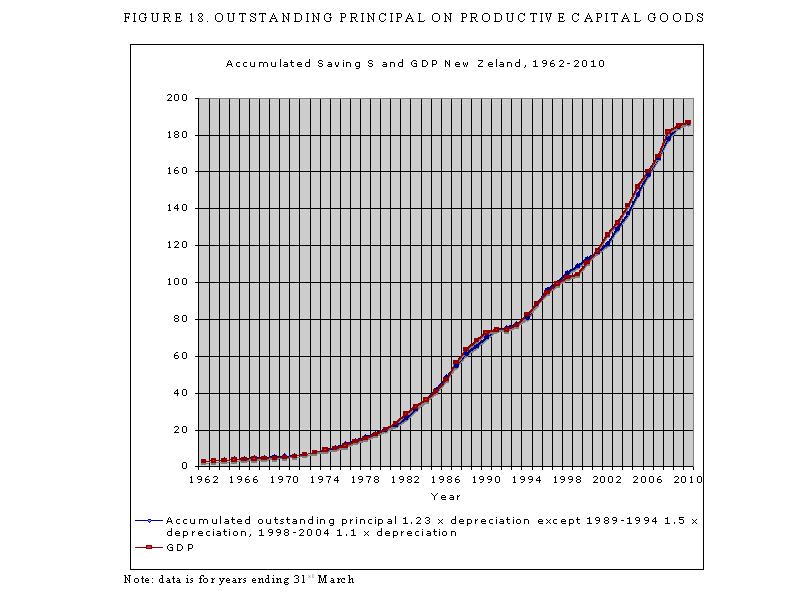
One reason for the
calibration is that the repayment factor of 1.23 x depreciation is an average.
It is not fixed and varies with the state of the economy. It will even vary a
little from one “ordinary” year to the next. 1990-93 was a time of severe
recession in
When (mostly new)
businesses fail their assets are sold off and some of the debt gets repaid.
That increases the outstanding principal repayments relative to the outstanding
debt, particularly when banks are forced to write down debt to cover losses or
when
they demand greater repayments
from businesses that have not failed. The reverse seems to have been the case
in
55. The
correspondence is very good even without the calibration because the effects of
lower Saving during the 1990-1993 recession and the higher saving during the
2000-2002 dotcom boom cancel each other out.
56. Narrower time frames (1990-1993, 2000-2002) could have been used in the calibration except the repayments 1990-1993 would have been 1.6 x depreciation and those 2000-2002 would have been 1.0 x depreciation. The calibration shown is considered to be appropriate pending further research.
Figure 18 shows
that with just the two calibration corrections over 62 years, the model
outstanding principal Is fits the official GDP data like a glove.
There were not many failures or bankruptcies in
There cannot be any
increase in production or GDP without an increase in productive investment I.
Increases in
productivity affect prices rather than GDP.
The accumulated
total I of productive Saving S equals the gross domestic product GDP.
National Saving S
calculated as the gross capital formation less principal repayment over any
period equals the nominal GDP increase over the same period.
Long-term business
economic profit equals the opportunity cost of capital as required by orthodox
economic theory.
A subsistence
economy requires little investment. The most valuable possessions of tradesmen
in medieval times were their (few) tools. Their tools were far more valuable
than their house and were often inherited.
In a modern
society, greater employment requires investment, in aggregate, for supervision,
equipment, transport and the like, even when capacity utilisation is relatively
low in the presence of unemployment. Orthodox economic theory insists that
unemployment rises when there is insufficient investment and (re)training to
provide the skills a developed economy needs. Figure 18 supports that view. It
suggests that existing capital investment must not only be replenished as it is
repaid, but must be extended if measured economic growth is to occur.
In the debt model
derived in section 8, the money to pay for the capital goods an economy
produces comes from incomes (compensation of employees and gross operating
surplus of businesses) generated through the production cycle. These are
reallocated for investment in capital goods as shown in Figure 11 of this
paper. Once the loan to purchase the capital good is in place, the production
loan is repaid as shown in Figure 11.
The entrepreneur
who has bought a capital good conceptually has a corresponding debt not to the
bank but to the rest of the productive sector. The loans are “real” but
notionally they do not affect the supply of new bank debt.
In practice, most
productive lending is now intermediated through the banking system as shown in
Figure 11. Bank intermediation allows non-productive “saving” to take place outside
the production system. Instead of “savers” borrowing to “save” as the
debt system requires, entrepreneurs borrow from the banks while income earners
and businesses “save” their share of the value of the capital goods they have
produced. Conceptually, the net effect
remains the same. Income earners and businesses lend to entrepreneurs and
borrow to “save” for their non-productive investments.
The main historical
reason non-productive saving is not equal to system deposits less the dynamic
production deposits My is that a lot of productive investment in New
Zealand used to be funded directly by borrowing the deposits of other deposit
holders (such as through solicitors’ trust accounts, insurance companies,
Masonic lodges, the Post Office Savings Bank, building societies, Stock and
station agents, non-bank finance houses) rather than through the banks. That
meant there were fewer deposits left over for unproductive “saving”. More
recently, consumer finance in the form of credit cards and hire purchase has
increased borrowing for consumption, allowing for some increase in unproductive
“saving”.
Debt and interest
payments covering new productive capital assets are repaid out of new income
generated by their use. That is the only feasible way to repay them unless new
debt is borrowed to repay existing debt and interest. Otherwise the production cycle could not
remain self-clearing.
Growth arises
directly from the additional production created using the new capital goods.
The entrepreneur must repay the loan he has conceptually received from his
co-producers and ALSO make a profit from the new investment to provide his own
income (part of his operating surplus). Otherwise there would be no economic
rationale in making the investment in the first place. That is why benefit to
cost ratios are sometimes applied when deciding to invest in capital assets. A
low benefit to cost ratio low indicates there will be insufficient profit from
the investment to provide the entrepreneur a satisfactory income after all
costs and repayments have been deducted.
Non-productive
capital assets like housing, including new housing, provide a repayment
challenge to those who buy them. Homeowners, for example, must often pay for
their home out of their (future) income. To do so in aggregate, they must
either increase their productivity over time in the hope their incomes rise in
real terms or there must be an adequate redistribution of income from the
business gross operating surplus to households through taxation.
The business sector
claims, with some justification, that redistributing entrepreneurial incomes
reduces productive investment. That would be the case if management salaries
and bonuses remained constant. In the debt model, using existing incomes for
debt repayment must result in loss of purchasing power, growing unemployment,
recession, and perhaps even deflation. In
To give a numerical
face to Figure
57. As stated above, the
accumulated total of productive Saving Sy equals the gross domestic
product, GDP.
According to
According to the
provisional model in Figure 18 the
The amount of
productive debt My used to actually produce the nation’s goods and
services is small. While My increases as the economy expands, it
remains at roughly just 5% of GDP because it reflects the nature of the payment
systems within the economy. It is “rollover” funding as set out in the debt
model (see Figure 14) and it presently has a speed of circulation in
As discussed above,
the loans (and interest) relating to new productive capital assets must be paid
from new GDP created by the new investment as shown in Figure 11, otherwise
there would be no point in making the investment in the first place. The new
production produces the additional employee and entrepreneurial (gross
operating surplus) incomes to consume the new production.
The ONLY new earned
purchasing power entering the productive system apart from utilisation of
existing unused productive capacity arises from added production from new
capital assets. Any other purchasing power would have to be borrowed as
“consumer finance” and would be inflationary unless it is used to offset
non-productive saving.
Since debt can be
used only once 58, higher employee and entrepreneurial incomes must
be a proxy for increased GDP.
58. My is conceptually recycled at the end of each production cycle.
If new capital
goods did not increase output, entrepreneurs would quickly become bankrupt because
there would be no income either to repay the loan they have taken out to
purchase the capital good or to pay the interest on it. Further lending by the
banks would then be withheld due to higher perceived lending risk. The system
dynamics would then fail, as happens during recessions.
Except by utilising
existing idle productive capacity, the only way to increase GDP is through new
productive investment so that GDP cannot increase faster than investment.
To be able to make
its debt repayments an economy must expand by at least the net amount of new
productive debt coming into the system, that is, the gross capital formation
less repayments 59.
The debt model
confirms the orthodox economic principle that in a competitive market economy
long-run economic profit is zero 60.
59. Additional interest on
the debt My appears to be a secondary
inflationary factor in the system.
60.
See for example Baumol and Blinder op cit Chapter 25. Zero economic profit refers to the situation
after the opportunity cost of capital is taken into account (represented in the debt model by interest on
the debt itself).
The debt-based
economy does NOT provide any way to repay the loans used to buy non-productive capital
goods such as residential housing using earned incomes because, by their
nature, such capital goods are mostly non-productive. There are intangible
benefits of good housing like better health, lower stress and proximity to work
but those benefits are not measured in the gross domestic product (GDP).
In aggregate, in
the interest-bearing debt system, housing debt is repaid through the exchange
of existing property and consequential capital gains in much the same way
revaluation and refinancing must be used to fund other non-productive
investment such as Kiwisaver in
In the present debt-based
economic system the housing market relies on investment sector inflation.
As long as the
accumulated current account balance is zero, and debt is expanded according to
the systemic needs of the productive economy described in the debt model set
out in this paper, asset prices will inflate more or less in line with nominal
GDP growth.
This can be
confirmed by considering equation (10) as it applies to a country like
d/dt DC = d/dt ( GDP/Vy - M0y + Ms + Dca
+ Db ) (10)
In creditor
countries like
d/dt
DC = d/dt (Ms + Dca )
If, as is the case
in
d/dt DC = d/dt
(Dca ) approximately.
When d/dt Dca is
negative, d/dt DC is also negative, and this is what has been causing
61. Ms itself is
far from zero because the massive property bubble in
62.
Figure 19 shows the
DNA of the debt-based economy. It shows how economic output (GDP) and Saving
are irrevocably linked in a twin helical structure with the one dependent
entirely on the other.
Figure 19 results
directly from the debt model based on the revised Fisher Equation of exchange
developed by the author and provided in this paper. Each conceptual production
cycle uses transaction funding My to produce goods and services. My
is a dynamic and continuously variable financial input that gives rise to an
equal value of output that includes earned employee incomes, the gross
operating surplus and indirect taxes.
Conceptually, that input is always just sufficient to clear the
market at current prices but changes to take into account inflation and
increased production as more non-financial economic resources (labour and land)
are utilised.
National Saving is
the difference between gross capital formation and principal repayments. For
the system to remain stable, Saving must be exactly enough to purchase the
capital goods produced in any cycle. That is why saving, investment and
economic growth are exactly linked as shown in the DNA diagram of the
debt-based economy in Figure 19.
Non-productive
“saving” occurs when National Saving is diverted to non-productive investment
in pension funds, Kiwisaver and ordinary term bank deposits in New Zealand and
replaced by new bank debt in the form of consumer debt or household revaluation
and refinancing. To the extent that
happens, bank debt increases. Instead of entrepreneurs borrowing the incomes of
employees and businesses earned through the production of the new capital
assets, those incomes are “invested” in non-productive investment and new bank
debt is used to fund the entrepreneurs instead. There is nowhere else for the non-productive
“saving” to come from, just as there is nowhere for the debt servicing and
repayments of new non-productive debt to come from.
The economic system
under the revised Fisher Equation is a closed system. With Vy now
more or less constant in many countries (Figure 14) the only way to increase
output at constant price is to increase My and, by and large, the
only practical way to increase My at full employment (model Db
= 0) is through productive capital investment. There may be a little leeway following
a recession when capacity utilisation, of both capital goods and labour, is
less than optimal, but even that will usually involve some investment and is
temporary. It would appear as a correction to Db in the debt model.
The balance between
incomes, output and purchasing power is absolute. The debt model does not allow
for economic multipliers.
Economic growth and
productivity can be improved by giving precedence to productive investment over
non-productive investment, and to the production of capital goods over
consumption goods. Moreover, there is ALWAYS a trade-off between
non-productive consumption, including non-productive government expenditure, on
the one hand and capital investment, including productive government
investment, on the other hand.
Figure 19 is made
up of two mirrored helical strands of DNA.
The blue strand represents the total accumulated GDP output while the
red strand represents the total outstanding investment principal. The vertical
axis of the helices represents time.
On the blue helix, Vy
bases of production output My are added over the time span needed to
make one full turn of the blue helix (usually a year). On the red helix, Vy bases of
national saving Sy (net new productive investment) are added over
the time span needed to make one full turn of the red helix (usually a year).
The helices therefore
replicate by extension. The blue helix
“dies off” at the end of each period
The helices grow by the
transfer of National Saving Sy from the blue helix to the red one
over each notional production cycle. There are Vy such cycles during
each period (usually a year)
For each of the bases, the
national saving Sy is returned to the next production cycle on the
blue helix in the form of net new capital investment Sy (Saving =
Investment) as shown.
The bases can vary in size (up
or down) according to the state of the economy.
The annual length or “growth
ring” Lz of the blue helix is the GDP for that year.
The nominal GDP growth in the
blue DNA is the change in length Lz of the DNA spiral over the
period z compared with the corresponding length L z-1 over the
previous period.
The annual length or “growth
ring” Lz of the red helix is the increase in outstanding investment principal
S which also equals the nominal GDP growth for that year.
The total length of the red
helix is the sum of all outstanding investment principal and it equals the
current nominal GDP at any time.
At the end of each (annual)
period z (and only then) the value of output represented by length Lz
of the blue helix (the GDP for that year) equals the value represented by the
whole of the red helix (the sum of outstanding investment principal that also
equals the GDP).
The plan diameter
of the helices typically expands exponentially. The helices are three
dimensional, so the diameter shown at the “crossing” points in the
two-dimensional diagram on Figure 19 is similar to that at all other points on
the curves after allowing for nominal GDP growth.
The helices vary together with
the state of the economy. In the case of recessions they show up as a reduction
in the rate of increase of the helix
diameter. In the case of depressions they show up as an actual decrease in the helix diameter.
Increasing productive
capacity means directly increasing My by directly putting spare
productive resources to use or developing new ones, or by better using existing
resources.
The mechanisms outlined in
this paper show why economic policy has failed until now. To expand the economy, My needs to
increase with little or no inflation so deposit interest rates need to be close
to zero and the quantity of new deposits needs to constrained without raising
interest rates. To expand My means increasing productive investment. To increase productive investment means the
increase in My must be directed into new plant, factories, training
and technology. At present, that means reducing consumption so as to increase
national saving, S.
One key way to do this is to
extend the repayment period for productive capital goods.
The combination of low or zero
deposit interest and extended repayment periods for capital goods will
transform national savings by drastically reducing debt servicing.
In addition to reducing the
burden of debt servicing on capital goods, interest-free funding can injected
to allow consumption to continue while using spare resources to increase
production capacity. One way to do this is outlined in Paper 3 (link provided
below). As that new productive capacity becomes operational it increases
productive efficiency and consumption capacity.
12.
SUMMARY.
Debt.
For practical
purposes, debt-based financial systems in modern industrialised countries are cashless.
In industrialised (and most other) countries, privately owned banks create new
debt and charge their clients for doing so. In the
debt-based system the debt is created before its corresponding money deposit.
Except for residual
cash transactions, in a debt-based financial system there is a unit (dollar) of
debt for every unit (dollar) of “money”. For every unit (dollar) “saved” by one
person there is a unit (dollar) of debt owed by another.
Debt can only be
used once. Once debt is used it must eventually be repaid with interest. Unless
it is written off by bank failure, existing debt can be repaid only by reducing
the banking system deposits or net worth.
Debt growth.
The debt based
financial system is dynamic and independent of orthodox economic equilibrium
theory. Orthodox economics offers no mechanism to achieve
elimination of unsustainable debt growth. As the ratio of unearned income to
GDP increases, the ability of the productive economy to fund the pool of
unearned income decreases.
Net after-tax
interest paid by banks on their clients’ deposits forms an exponentially
increasing pool of non-productive unearned interest income that is never repaid
and is a structural part of the debt-based financial system. The interest rate
on deposits must be eliminated if the exponential growth of the pool of
non-productive unearned income is to be stopped. Unless the deposit interest
rate is zero, Domestic Credit, unearned deposit income and nominal GDP must all
grow exponentially because, in the debt based financial system, they are all a
function of the deposit interest rate.
In the absence of
realised capital gains it is impossible to maintain exponential debt expansion
greater than GDP expansion over an extended period because the added debt
servicing costs will always leave the productive sector insolvent. The debt
supporting the exponentially increasing pool of non-productive unearned income
leads to an ongoing transfer of real wealth from the productive sector to the
non-productive investment sector.
Credit bubbles, recessions and depressions result from the failure of
the banking sector to properly align demand for credit with the productive
capacity of the economy. Credit expansion in the banking system above what the
debt system requires means there is a bubble in the economy while credit
expansion below what the debt system requires means there is a recession or
depression in the economy. A credit bubble or economic contraction is
neutralised when credit expansion has been adjusted so that it just satisfies
what the debt system requires taking into account the full productive capacity
of the economy.
There is no “money”
multiplier in the debt based financial system other than the (slightly) variable speed of circulation of
the transaction deposits actually used to generate productive economic output.
Exponential debt growth can be eliminated by progressive credit
monetisation of the existing debt and by permanently reducing the OCR (Official
Cash Rate) towards zero, at which point systemic inflation caused by interest
paid on deposits would be removed from the financial system.
Inflation.
Systemic inflation
and exponential debt growth are caused by interest paid on bank deposits.
Interest paid by banks on their clients’ deposits forms an exponentially
increasing pool of non-productive unearned income that is a structural part of
the debt- based financial system and cannot be repaid.
In a debt-based
economy where interest is paid on deposits, systemic inflation is half the interest
rate paid on deposits provided adjusted wage rates rise in line with that
systemic inflation plus productivity growth and there are no changes to
indirect taxes. Systemic inflation arising from deposit interest automatically
reduces towards zero as deposit interest rates reduce towards zero. However, in
the absence of quantity controls on the issue of new debt, low interest rates
can lead to unproductive “bubble” lending, thereby increasing price inflation.
In an economy based
on interest bearing debt, almost all price is inflation. Aggregate consumer
prices inflate with the deposit interest rate so that deposit interest on
existing productive investment can be paid into the unearned income pool
without disrupting the productive economy. Increasing interest rates to manage
inflation increases the flow of deposits from the productive sector to the
investment sector by increasing the unearned income pool. It is no longer possible to combat inflation
by substantially increasing interest rates (or to stimulate growth by reducing
them) because modest increases in interest rates are now enough to drive the
economy into recession.
Foreign ownership
of a part of a debtor economy causes asset inflation there because there are
more domestic deposits available to fund the exchange of assets remaining in
domestic ownership.
The supply of new electronic cash (not debt) to businesses to fund
virtual increases in minimum wages does not necessarily cause immediate
increases in prices because the E-Note injections are not part of production
costs and some of the extra wages will be used for private debt retirement.
Banks.
In a debt-based
system, the interest banks charge their clients to provide goods and services
(the bank spread) is part of productive economic activity and does not cause
inflation. When the bank spread and costs are constant, the larger the total
debt of a nation the larger the turnover of the banks and the more profit they
make.
Deposit interest paid by banks to their
clients is not specifically beneficial to the banks but is the fundamental
source of systemic inflation in the debt-based financial system. Public credit
and money issue enables domestic banking systems to operate in high growth, low
risk, low interest, low inflation economies while retaining their existing
profit margins.
Gross domestic product (GDP).
The nominal
increase in GDP over any period equals the increase in National Saving, which
is the gross capital formation less principal repayments over the same period.
Productivity growth
is inherently deflationary. It usually affects prices rather than GDP and
declines as an economy becomes more service-based. Except by utilising existing
idle productive capacity, the only way to increase GDP is through new
productive investment through the supply of new transaction deposits to make
use of spare labour and resources in the economy or to increase the skills of
and re-employ existing resources, and by the relationship between the
production of capital goods and goods and services for consumption
Interest rate
reductions stimulate an economic recovery only when the capital gains from the
exchange of existing capital assets produce enough new debt to satisfy the
systemic debt requirements of the financial system.
In a cash-free debt
based economy with zero interest rates on deposits the increase in GDP equals
the speed of circulation of debt in the productive sector times
(a) the change in
domestic credit, less
(b) the current
account deficit, plus
(c) a correction
for any imbalance between the change in domestic credit and what the debt
system requires taking into account the full productive capacity of the economy
Business cycles.
A recession
provides for inflation but not economic growth, while a depression provides for
neither economic growth nor inflation. A recession occurs when the change
(increase) in the total debt (both public and private) over time is less than
what is needed to service the financial system costs made up of the net
unearned interest that has to be paid on all bank deposits plus any new current
account deficit plus any increase in the productive debt used to generate new
economic output. A depression is a deep recession that also fails to provide
for inflation.
Income distribution.
Apart from utilisation
of existing unused productive capacity, the additional production from new
capital assets is the ONLY way to increase earned purchasing power in a
debt-based economy.
The SHAPE of an economy, which is the basket
of goods and services produced in relation to incomes and consumption patterns,
is largely determined by its income distribution. Poor income distribution
suppresses demand for domestically produced goods and services. Since the employed workforce is already
producing goods and services, the SHAPE of the economy must change to
improve economic efficiency and promote
domestic production.
Socially mandated
income redistribution is necessary to distribute productivity increases throughout
the economy and improve real wages and purchasing power. The application of a
single flat financial transactions tax to all withdrawals from bank accounts
changes the shape of the economy by redistributing income.
Taxation.
Skewed tax systems benefit
a relatively small section of society at the expense of everyone else because
they impair economic performance and economic growth potential by systemically
transferring purchasing power from the productive sector to the unproductive
sector through increased debt and debt servicing.
A uniform wealth tax on all net wealth from all sources is
redistributive because it (gradually) reverses the accumulation of net wealth
inherent in the presently dominant debt-based financial system. A single Financial
Transactions Tax (FTT) automatically
collected on withdrawals from bank deposits can help correct the tax skew
inherent in existing taxation systems that substantially exempt the investment
sector from paying its “fair share” of tax.
Consumption (with housing).
Most residential
housing is economically unproductive once it has been built, thought its
construction is part of the productive economy. Residential housing that does
not generate income is incompatible with a financial system based on interest-bearing
debt.
Assuming incomes are constant and there are no productivity gains or
realisation of capital gains through asset inflation, homeowners must reduce
their domestic consumption by an amount equal to the principal and interest
payments they make on their non-productive capital assets. The reduction can be
(partly) offset through capital gains. Realised values from the
exchange of existing assets must in that case increase by an amount sufficient
to cover both the interest and principal repayments. The reduction in domestic
consumption must otherwise be matched by the export of the
resulting surplus consumption goods and services if structural employment and
recession are to be avoided
The process of production and consumption in the
productive economy is self-cancelling wherever it takes place and however its
phases of production and consumption are shared amongst nations. Export of surplus consumption goods and services to avoid structural
unemployment and recession decreases foreign ownership of the domestic economy.
It does not directly improve domestic wellbeing in the exporting country.
Inclusion of a
housing provision in a tax-free guaranteed minimum income (GMI) system allows close matching of the GMI
to existing government income transfer structures in many industrialised
countries
Capital formation.
Capital formation
in a debt-based economy takes place in accordance with the basic tenet of
orthodox economics that National Saving equals Productive Investment. It arises
from the redistribution of employee income and gross operating surpluses of
businesses to purchase the capital goods created by the productive economy.
Production must always, but only just, lead consumption to provide the incomes
that enable consumption to take place.
Saving.
In the modern
world, faster depreciation has swapped longer-term productive investment to
boost existing stock and existing property prices. Saving for productive investment and real GDP
growth as measured using the international System of National Accounts cannot
be restored to modern developed economies unless the protocols around
depreciation are altered, bank lending polices and regulations reviewed and the
serious distortions in the System of National Accounts (SNA) records themselves
are corrected.
In a debt-based
financial system and in the absence of a debt bubble it is impossible to
increase National Saving (and therefore GDP) without increasing production
loans and new productive investment. In the absence of asset inflation, any
attempt to withdraw any part of deposits for non-productive investment purposes
(“savings”) reduces purchasing power in the productive economy or leaves
capital goods unsold, leading to increases in inventory, and subsequent
unemployment and recession. Unproductive savings and pension schemes such as
Kiwisaver in
Investment.
The investment
sector represented by the accumulated net after tax interest paid on bank
deposits produces nothing itself and is paid for through inflation in the
productive sector. Increased depreciation allowances speed up principal
repayments and reduce national saving and productive investment. Increased
repayment of debt, including household debt, reduces national saving and
reduces net new productive Investment.
The accumulated net outstanding principal invested in productive capital
goods is equal to the net accumulated national saving because in a competitive
market economy the long-run economic profit of business tends toward zero as
profit falls toward the opportunity cost of capital. Productive investment
represents the redistribution of production incomes to clear the capital goods
market in the productive sector.
Economies in
recession must be stimulated by direct investment in new production because the
lead-time before the benefits of increased productivity from infrastructure
investment exceed the infrastructure costs is usually too long to be effective.
System of national accounts.
The
use of depreciation for measuring economic success has been catastrophic for
the world economy.
When the current account
balance is included as income in the national income and outlay account of the
SNA an entry of equal value entitled “purchase of capital assets on the current
account” should be included on the other, “use of income”, side of the national
income and outlay account.
The National income
and outlay account of the SNA needs to be restructured and the National capital
account consequentially adjusted to reflect orthodox economic theory as
follows:
Use of income side:
= Final consumption C
+ Purchase abroad of non-productive
capital investment goods (=CA)
+ Saving for productive investment S
Income side:
= GDP
+ Current account balance (CA)
less the balance on external
goods and services
less repayments of principal
on outstanding productive investment.
Current account.
Current account transactions are exchange
transactions, not production transactions. To avoid bankruptcy of the
world economy in the long run, each nation must maintain, in aggregate, a zero
accumulated current account.
There is no such
thing as foreign debt; there is only foreign ownership by foreign creditors of
part of a debtor’s nation’s economy either as physical ownership or ownership
of commercial paper. An accumulated national current account deficit reduces
national savings and increases the domestic debt of the debtor country, its
domestic inflation and foreign ownership of its economy. Foreign ownership of a
debtor nation’s economy drains its domestic economic growth through outgoing
current account payments of interest on commercial paper and dividends and
profits arising from the physical foreign ownership of its assets.
The debtor status
of debtor countries can only be managed without affecting their domestic
economies if their exchange rates are reduced so their current accounts become
positive enough to reverse the foreign ownership of their assets. In the absence
of effective management of capital flows and the exchange rate, the logical
outcome of the existing debt system in heavily indebted debtor countries is
national bankruptcy because debtor countries are condemned to paying high
interest rates to avoid capital flight.
Exporting domestic
production (“export-led recovery”) is an unsatisfactory method for reducing an
accumulated current account deficit unless the accumulated deficit is small and
the exchange rate is free to fluctuate independently of domestic interest
rates.
At any point of
time, the current account deficit in heavily indebted debtor countries is
typically just a little more than:
a) the accumulated
current account deficit of the debtor country, multiplied by the average bond
rate in the debtor country, minus
b) the trade
balance of the debtor country for the period, plus
c) the net
repatriated profits of foreign-owned banks operating in the debtor country over the same period.
A positive balance on
external trade swaps domestic growth in the exporting country for foreign
assets in the debtor country and is a positive growth factor for the exporting country’s business
interests. The logical outcome of the existing debt system in creditor
countries is zero deposit interest and stable or falling asset prices (as in
A tax-neutral variable
Foreign Transaction Surcharge (FTS) applied to all outward exchange transactions allows the progressive reduction in foreign ownership of the domestic
economy (the so-called foreign debt) by enabling the exchange rate to fall towards a
stable base level, increasing the value
of exports and decreasing the quantity of imports, and providing a more even
playing field for local manufacturers and producers.
E-notes.
Existing privately
issued interest-bearing government debt can be progressively retired as it
matures and replaced with publicly issued interest-free debt or E-notes spent
into circulation by the Government. E-notes (electronic cash) perform exactly
the same role as existing bank debt.
Zero or low interest credit and money issue
enables economic growth to be tied to the productive economy instead of being
inflated by deposit interest.
Local money systems.
Local money systems
are co-operatively owned interest-free, self-cancelling monetary systems in
which there is no systemic debt because the debt incurred during the production
phase is cancelled when the product or service is sold. They can be organised
nationwide and taxed in formal currency, promote domestic production, increase
economic efficiency and reduce financial leakage from local economies.
THE REFERENCED PAPERS
The
referenced papers :
NEW Capital is debt.
NEW Comments on the IMF (Benes and Kumhof) paper “The
Chicago Plan Revisited”.
DNA of the debt-based economy.
General summary of all papers published.(Revised edition).
How to create stable financial systems in four
complementary steps. (Revised edition).
How to introduce an e-money financed virtual minimum wage
system in New Zealand. (Revised edition) .
How
to introduce a guaranteed minimum income in New Zealand. (Revised edition).
Interest-bearing debt system and its economic impacts.
(Revised edition).
Manifesto of 95 principles of the debt-based economy.
The Manning plan for permanent debt reduction in the national economy.
Missing links between growth, saving, deposits and
GDP.
Savings Myth. (Revised edition).
Unified text of the manifesto of the debt-based
economy.
Using a foreign transactions surcharge (FTS) to manage the
exchange rate.
(The
following items have not been revised. They show the historic development of
the work. )
Financial system mechanics explained for the first time. “The Ripple
Starts Here.”
Short summary of the paper The Ripple Starts Here.
Financial system mechanics: Power-point presentation.
Return to : Bakens Verzet
Homepage
"Money is not the
key that opens the gates of the market but the bolt that bars them."
Gesell, Silvio, The
Natural Economic Order, revised English edition, Peter Owen,
This work is licensed
under a Creative
Commons Attribution-Non-commercial Share-Alike 3.0 Licence.