NGO Another Way (Stichting Bakens
Verzet), 1018 AM
SELF-FINANCING,
ECOLOGICAL, SUSTAINABLE, LOCAL INTEGRATED DEVELOPMENT PROJECTS FOR THE WORLD’S
POOR
|
FREE
E-COURSE FOR DIPLOMA IN INTEGRATED DEVELOPMENT |
|||||
Edition 02 :22 July, 2013.
(VERSION EN FRANÇAIS PAS DISPONIBLE)
Summaries of
monetary reform papers by L.F. Manning published at http://www.integrateddevelopment.org.
Chicago Plan Revisited Version II: An insufficient
response to financial system failure. (Posted 11 May, 2013.)
Comments on the (Jaromir
Benes and Michael Kumhof) Chicago Plan Revisited Paper.
Debt bubbles cannot be popped : Business cycles are policy inventions.
DNA of the debt-based economy.
General summary of all papers
published.(Revised
edition).
How to create stable financial systems in four
complementary steps. (Revised edition).
How to introduce an e-money financed virtual minimum wage
system in New Zealand. (Revised edition) .
How
to introduce a guaranteed minimum income in New Zealand. (Revised edition).
Interest-bearing debt system and its economic impacts.
(Revised edition).
Manifesto of 95 principles of the debt-based economy.
Manning plan for permanent debt reduction in the national economy.
Measuring Nothing on the Road to Nowhere.
Missing links between growth, saving, deposits and
GDP.
Savings Myth. (Revised edition).
There’s no such thing as affordable housing.
Unified text of the manifesto of the debt-based
economy.
Using a foreign transactions surcharge (FTS) to manage the
exchange rate.
(The
following items have not been revised. They show the historic development of
the work. )
Financial system mechanics explained for the first time. “The Ripple Starts
Here.”
Short summary of the paper The Ripple Starts Here.
Financial system mechanics: Power-point presentation.
![]()
This
work is licensed under a Creative
Commons Attribution-Non-commercial-Share Alike 3.0 Licence
MEASURING NOTHING ON THE ROAD TO NOWHERE: THE
MYTHS OF INFLATION AND GROWTH MEASUREMENT.
By
Sustento Institute, www.sustento.org.nz
July, 2013
email:
manning@kapiti.co.nz
This
paper shows conclusively that the existing world economic order is approaching
a state of structural collapse as the sum of accumulated systemic inflation (Ms
in the paper) plus the bank residual (R in the paper) approaches nominal GDP
leading to debt default and the destruction of GDP.
The
policy response to such a systemic collapse requires all of:
(a) Reducing
deposit interest rates toward zero [in progress]
and
(b) Managing the money supply
and
(c) Controlling cross border capital flows
and
(d) Stimulating productive investment
and
(e) Reversing income inequality.
Paper
released 9th July 2013.
EXECUTIVE SUMMARY.
More people working
efficiently for more hours increase productive output. The same people working
more efficiently for the same number of hours increase their productivity. Both
are forms of economic growth. Orthodox economics generally discounts real
productivity gains and fails to effectively measure economic growth. By using
the basic accounting equation and the debt model described in the paper,
economic “growth” can be better managed without creating the boom and bust
cycles that are typical of orthodox approaches to money supply. The paper
suggests there are few measured productivity gains in the debt-based financial
system. All “price” is inflation and most nominal GDP increases now represent
systemic inflation.
The paper also shows how
productive sector consumer price (CPI) inflation is misrepresented in key
economic data. CPI inflation measured as an increase in consumer prices over
time cannot simply be subtracted from the nominal increase in the value of
Gross Domestic Product (GDP) to provide an economic “growth” figure because the
average percentage “value” of inflationary increases in GDP is only half the
percentage CPI price rise.
Since the
Neither approach has worked
because neither approach satisfies the basic accounting equation given in
equations (1) and (2) discussed in this article, resulting in decades of poor
economic outcomes and devastation for countless millions of people around the
world.
BACKGROUND.
Recently, there has been a
great deal of discussion about a monetary reform program called the Chicago
Plan. The IMF has modelled that proposal in a working paper called “The Chicago
Plan Revisited” (CPRII) ( see Jaromir Benes & Michael
Kunhof, IMF working paper WP/12/202
final version 12th February, 2013). The proposal entails replacing existing interest-bearing
bank debt with debt-free, interest-free money called Treasury Credit in an
effort to stabilise the world’s monetary system. The CPRII modelling uses a
Friedman nominal money growth rule formula (CPRII equation 31, and p.61 top)
for the reformed monetary system. That controls inflation in the productive
sector only if just the right amount of new money is allocated to the
productive transaction accounts used to generate “optimal” economic output. As
discussed below, setting money growth equal to a subjectively established
growth rate of output is insufficient in a debt-based system, whether that debt
is bank debt or secondary (Savings and Loan) debt. Benes and Kumhof also use a
“conventional forecast based interest
rate [
This paper suggests the Friedman
money rule and
Figure
1 shows M3* 0.945 and GDP plotted against time for
Due mainly to the increase in New Zealand’s negative
net foreign currency assets, the investment sector in New Zealand has grown at
5.9%/year while its nominal GDP has grown at 5.2%/year over the same period.
That is partly why prices in the non-productive investment sector there are
“overvalued” and why neither the Friedman rule nor the
[Figure 1.
The author’s paper the DNA of the debt-based
economy demonstrates that GDP equals the outstanding
principal on productive capital investments (fixed capital formation). Were the
growth of 0.945* M3 to exactly follow the growth of nominal GDP, the prices of
existing assets in aggregate would
closely mirror nominal GDP.
The reasons why the Friedman
and Taylor rules cannot apply, and the myths underpinning present inflation and
growth measurement are now discussed.
THE RELATIONSHIPS BETWEEN MACROECONOMICS AND THE BASIC ACCOUNTING
EQUATION.
Dollar references in this paper are to the
It is impossible for deposits to be lower than the existing
interest-bearing debt in the capitalist system after subtracting the country’s
net foreign currency debt and the banks’ net worth that they have “captured”
from the deposit base. Otherwise the basic accounting equation (1) below is not
satisfied.
Debt is linked to deposits, the current account and capital transfers by
equation (1) :
(DC + NFCA) = M3 + Residual (R) (1)
Assets = Liabilities
+ Net
worth
The formula in equation (1) represents the basic accounting equation. The Residual is positive in the equation (1) format, while NFCA is negative for debtor countries.
Equation (1) can easily be
expressed for the post CPRII monetary reform proposed in The Chicago Plan and
other financial reform proposals using debt-free, interest-free money, as in
equation (2):
Assets = Liabilities +
Net worth.
Treasury Credit + Residual debt + NFCA
=Deposits + Residual (R) (2)
In equations (1) and (2):
DC =
Domestic Credit.
NFCA =
Net Foreign Currency Assets of M3 institutions plus those of the Reserve
Bank ( in
(RBNZ)).
M3 =
Deposit liabilities of M3 institutions plus those of the Reserve Bank ( in
Residual R = Aggregate retained bank profits
+ paid up capital.
Treasury Credit =
Debt-free, interest-free central bank credit.
Residual debt = The
sum of [remaining bank debt during the reform transition period + any central
bank lending to banks or investment
trusts for
government and private productive capital investment].
Equation (1) is the basic accounting equation stated from the banks’
point of view.
In
The orthodox
(Friedman and Taylor type) monetary policy rules fail because they consider
only the productive economy whereas they have to satisfy the basic accounting
equation (equation (1)) that also includes the non-productive investment
sector, the accumulation of bank net worth and the external investment
position.
In contrast to orthodox
economics, the author’s modified Fisher Equation of exchange fully satisfies
equation (1). It is :
DCm
=(GDP)/Vy +Ms +Dni +Db+R - Dnfca+Nb (3)
Where:
DC = Domestic Credit.
DCm = Domestic Credit plus secondary debt Nb borrowed
through non-bank lending institutions (NBLI). (DC = DCm-Nb).
GDP/Vy = The debt and cash used to create GDP
(Dmy= Dmt+M0y).
GDP = Gross Domestic Product.
Vy = The speed of circulation
of productive transaction accounts.
Dmy = The productive transaction
account balance used to generate GDP.
Dmt = The portion of Dmy
arising from bank debt.
Dni = Debt
supporting non-inflationary economic growth.
M0y = The portion of Dmy
contributing to the non-inflationary cash transactions M0y * Vy
. (M0y * Vy is
included in Dni).
Ms = Accumulated systemic
inflation arising from net after tax deposit
interest paid on the total system debt DCm.
Dnfca = Net foreign currency assets resulting
from the current account and capital transfers from the rest of the world.
Db = Bubble debt (debt in
excess of the systemic debt requirements).
R = Bank residual retained profits and paid up
share capital not being part of the money supply M3.
Nb =
Secondary non-bank debt.
Note that the original version of the equation has been updated because
it erroneously incorporated the whole of the accumulated current account
deficit in the model instead of NFCA as required by equation (1).
The modified Fisher Equation (3) is reconciled with the basic accounting
equation as shown below:
(DC + NFCA) = M3 + Residual
(R) (1)
Assets =
Liabilities + Net worth
Where :
NFCA = The net foreign currency
assets of the M3 banking institutions and the central bank.
DC =
Domestic Credit = DCm
-
M3 =
Deposit base of the M3 banking institutions.
The formula represents the basic accounting equation, where DC is Domestic Credit plus secondary non-bank debt, M3 is the total bank deposits, NCFA is the Net Foreign Currency Assets of the banking system and Residual is the net worth of the banking system. The Residual is positive in the equation (1) format, and NFCA is negative for debtor countries.
Substituting the terms from equation (3) into equation (1) gives:
Assets = Liabilities + Net worth
DCm =[GDP)/Vy +Ms +Dni
+Db +Nb ] + R - Dnfca (3)
(DC + Dnfca) =[ Dmy +Ms +Dni
+Db +Nb]
-Nb + R (4)
Where from equation (1):
M3 = [Dmy+ Ms +Dni
+ Db] (5)
Figure 2 shows the main
elements of the author’s debt model.
Statistics are publicly available for all the variables in equations (4)
and (5) except for Vy, Ms Dni and Db.
Initially, empirical estimates have to be made in the
calculation of Ms and Vy because the physical data for
them is not yet directly available. There is no reason, however, why data for Ms
and Vy cannot be physically collected. The model is validated by
solving equation (4) or (5) for Dni and Db as shown in Figure 4
and Figure 6.
Equations (4) and (5) require
no other multipliers or assumptions.
Since the productive investment account balance (My)
used to generate GDP can be estimated by analysing physical cash flows in the productive
economy, a straightforward application of equation (3) will produce the
“bubble” debt Db as a residual once Dni has been
estimated. A positive rate of change of Db indicates bubble
formation in the economy while a negative rate
of change means bubble decay. Dni
can be calculated using equation (9). A key objective of macroeconomic policy
settings is to ensure Db = 0, that is, that there is just enough
debt growth to provide for the system costs (investment sector, plus productive
sector inflation) and support the cash-based transactions and other
non-inflationary increases in the economy.
[Figure 2.
The Schematic Debt Model.]
There is another crucial relationship developed by the author. This is
referred to above. In a debt-based financial system:
[GDP]=Outstanding debt
principal on productive capital investment. (6)
Equation (6) implies that the minimum theoretical domestic credit
DC required in the present debt system to support the productive
economy is:
DC = GDP/Vy
+ [GDP ] (7)
Suppose now that Dnfca and Db were zero as
“assumed” by the Friedman and Taylor rules. Cancelling the zero terms in
equation (4) (bearing in mind that Dnfca is the debt representing
NFCA, and Dmy is the debt representing GDP/Vy ) leaves in
that special case:
(DC + Dnfca) =[ Dmy +Ms +Dni
+ Db] + R (4)
DC
= GDP/Vy+ Ms + Dni + R (8)
Comparing equations (7) and (8) leaves in that special case:
GDP/Vy + [GDP] = GDP/Vy
+ Ms +Dni + R
[GDP] =
Ms +Dni + R (9)
In the special case of no
foreign debt and no bubble, GDP comprises systemic inflation Ms that
incorporates new debt to fund inflation, plus
new debt Dni to fund non-inflationary growth, plus the non-circulating bank residual
R. When Dnfca and Db are non-zero, DC, GDP and the terms
in equation (9) will vary because they are each dependent on the size of DC.
The debt model enables the effects of price (P) and output (Q) which
together form GDP to be studied in a way that orthodox economic seems to be
unable to do. As discussed later on, orthodox economics is
also mismeasuring productivity increases.
The debt model is far from radical. It is simply a revision of the original
Fisher equation of exchange still applicable to the productive economy:
M*V =
P*Q : [in the debt model (My * Vy = GDP)] (10)
Where:
M = money supply.
V = speed of circulation of M.
Q = output of goods and services.
P = price level.
Several important consequences follow from the revised Fisher equation
model and from the equations referred to above. The points discussed below are
not in order of priority.
Accumulated Current account
deficit plus capital transfers from abroad and the Net Foreign Currency Assets
of the banking system (NFCA).
The accumulated current
account and direct capital transfers from the rest of the world play a key role
in economic performance because the Net Foreign Currency Assets form part of
the money supply M3. On the other hand, accumulated deficits on a current
account deficit and capital transfers increase foreign ownership of a debtor
country’s economy, making the current account itself more difficult to manage.
Capital inflow (NFCA) increases the money supply M3 in the receiving (creditor)
country, increasing systemic inflation Ms there, and vice versa for
a debtor country. There are no “ifs” or “buts” about this.
The only practical way for
debtor countries to overcome this problem is to reverse foreign debt growth
using an effective tool such as a Foreign Transaction Surcharge (FTS) proposed
by the author to manage capital flows. [ For more information see Using a foreign transactions surcharge (FTS) to manage the
exchange rate.] It cannot be done by monetising the foreign debt
because while doing that might lower the exchange rate it also inflates
domestic costs, negating the benefit of the lower exchange rate.
Current accounts also dominate
the domestic interest rate structure in debtor countries because foreign
investors have to be encouraged to buy and own the debtor country’s assets. The
debtor country has to “compete” with the rest of the world to attract that
investment by offering relatively high financial returns. Since the domestic
systemic inflation Ms is the net interest paid on the
Domestic Credit (plus the net interest on Nb), domestic inflation
cannot be properly managed in the presence of substantial interest-bearing
foreign debt. Many economists will claim
That makes “free trade”
proposals like the Trans Pacific Partnership Agreement (presently being
negotiated in secret) suicidal for the domestic economy of debtor countries
unless they provide for effective control of capital flows in the national
interest.
They don’t.
Productive
Sector Inflation.
Domestic Credit (DC) and secondary
debt (Nb) must typically be funded from the productive economy. In
this paper,
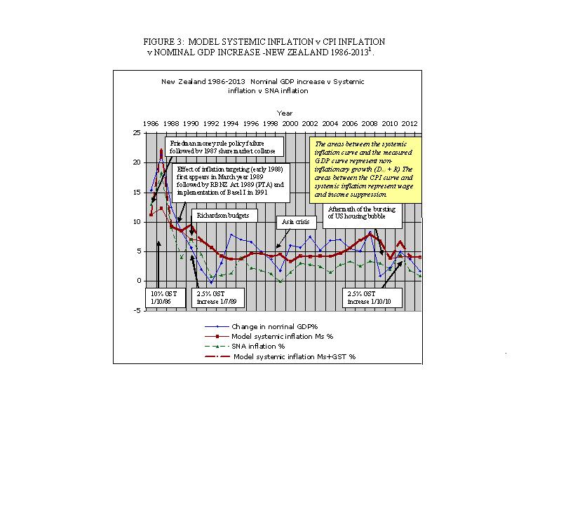
Domestically, cost-push
inflation is systemic and is the net deposit interest Ms
shown as Model Systemic Inflation in Figure
3. In
The main methodological issue
in calculating Ms is working out the net tax payments on the
interest because the tax represents a transfer payment to the government and so
remains in the productive economy. The effective tax rate on those receiving
deposit interest is the average tax rate paid over all the tax-payer’s income,
not the top marginal tax rate applied to that tax-payer’s income. Accurate
estimation of the net aggregate deposit interest lies beyond the scope of this
paper and is subject to further research. The NZ Department of Inland Revenue
can provide data on the tax paid on each income band and the numbers of people
in each band. An accurate assessment of tax may therefore be possible but it is
complex. In practice, it may be better to create new reporting and data series
to accurately calibrate the debt model deposit interest. The model is fairly
sensitive to the tax rate, so Figure 3 is preliminary
pending further work on the tax deductions on gross deposit interest.
Managing productive sector inflation
depends on eliminating deposit interest as far as possible. That is why
measured CPI inflation is very low in countries like
[Figure 3 : Model Systemic Inflation v. CPI Inflation v. Nominal
GDP increase New Zealand 1986-2013.]
Deposit interest rates used
to calculate systemic inflation are from Reserve Bank of
GDP
could be managed by changing the financial system to minimise systemic
inflation by reducing interest rates toward zero, and by managing the money
supply to fully utilise the physical economic resources available to the
economy, greatly reducing CPI inflation.
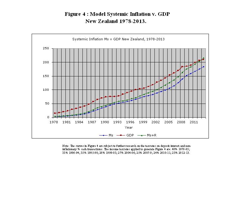
Since the debt model requires
exponential debt growth, Ms is also an exponential function. Figure 4 shows that the
accumulated inflation-free GDP component has been shrinking as a proportion of
GDP in
[Figure 4 :
Model Systemic Inflation v. GDP
Figure
4 suggests Dni has all-but disappeared
in
Figure 4 shows why real
incomes in many developed economies have been stagnant or falling in recent
decades. As shown later on (using the Fisher equation of exchange), the real
impact of systemic inflation is being masked by the suppression of
incomes.
There has been no aggregate
real growth in
Zero
Deposit Interest is Impossible in a Capitalist System.
GDP in the debt model is the net
outstanding principal on productive capital investment (fixed capital
formation). The reason this is so is set out in the author’s paper the DNA of the debt-based economy. In the capitalist system there must be debt
to enable the purchase and exchange of capital goods.
In a reformed financial system based on debt-free money, the money to purchase and exchange capital goods is borrowed from deposit holders at interest on a Savings and Loan (S&L) basis instead of from commercial banks. Consequently, there must be an “incentive to save”, otherwise there will be leakage from investment sector to the productive sector causing very high demand-pull inflation in the productive sector. In fact, all the main monetary reform proposals such as the Chicago Plan (CPRII), the Manning plan for permanent debt reduction in the national economy, the Positive Money proposal in the UK, and the AMI proposal in the US feature S&L lending.
When deposit interest rates are
close to zero, demand-pull inflation is limited only when savers choose to
hoard for a rainy day despite receiving little or no deposit interest (as was typical
in pre-industrial times), or where they choose to invest in dividend-bearing
investments or in direct productive investment for profit. This is commonly
called the “opportunity cost” of capital. A major difference between the modern
economy and that in pre-industrial times is that the relative amount of “saved”
money in the investment sector is proportionately much greater now than it used
to be.
With low interest rates and systemic
inflation there would be little property speculation because there would be
little aggregate capital gain. Instead, the investment property market would be
governed by the net return on investment such as, for example, net rental
income.
The core solution to rising
property and equities prices around the world is therefore to manage the debt and
money supply while reducing deposit interest rates to a level just sufficient
to provide an “incentive to save”. The only proposal currently complying with
the debt model and the accounting equation that does this is the author’s “The Manning plan for permanent debt reduction in the national economy.”
MEASUREMENT
OF GROSS DOMESTIC PRODUCT (GDP).
Orthodox economics divides the
increase in the nominal value of GDP into two parts: “inflation” and “growth”. In the original Fisher equation of
exchange, (equation 10), that still applies directly to the productive sector
in the debt model, changes in output on the variables (using Newtonian
notation), assuming speed of circulation Vy is constant, are given
by:
(My + dMy/dt)
*Vy = (Q + dQ/dt) * (P +
dP/dt) (11)
Therefore:
(P + dP/dt) =
((My + dMy/dt) / (Q + dQ/dt)) *Vy (12)
and the price increase:
dP/dt = ((My
+ dM/dt) / (Q + dQ/dt)) *Vy – P (13)
If there is no price change,
(dP/dt = 0). Then:
P=1 =
(My + dMy/dt) / (Q + dQ/dt) *Vy (14)
Suppose Vy =
10, My=100, Q= 1000/year
and P=1.
If dMy/dt changes
by 20, to maintain P=1, dQ/dt must
change by 200 because from equation (14)
P =
(My + dMy/dt) / (Q + dQ/dt) *Vy (14)
1 = (100+20) /
(1000+200) *10
At
constant price and speed of circulation, producing 20% more goods requires 20%
more money, that is, wages and incomes. Changes
in productive transaction account money My and output Q are always
and necessarily proportional when P and Vy are constant.
If, on the other hand, there
is an annual 10% increase in prices, (dp/dt = 10%/ year), to get the same rate
of output at the end of the year requires:
P =
((My + dMy/dt) / (Q + dQ/dt)) *Vy (14)
1.10 = (100+31 ) /
(1000 +200) *10 at year end
1.10 = (131) / (1200) *10 at year end
The Fisher equation presented
here is a macro-economic snapshot at a point in time. At the end of the year
the goods in the example are being produced at the rate of 1200/year
when the productive transaction account money supply is 131 (instead of 120)
and prices are 10% higher than the previous year. However, the situation over
any period is dynamic, not static. All the variables are increasing over time
so they have to be “averaged” over the period in question when using the annual
output measure of GDP.
In the example, at the end of
a full year when P=1.1, there is then a rate of production 1200/year. During
the year, 1100 goods,[(1000+1200)/2],
have been produced at an average transaction account money supply M of
115.5 [(100+31)/2] and a linearly averaged price of 1.05 as shown below:
P =
(My + dMy/dt) / (Q + dQ/dt) *Vy (14)
1.05 = (100 + 15.5) /
1100* 10 averaged
and:
GDP (PQ) = My*Vy
1.05*1100
= 115.5*10
1155 = 1155
The real annual GDP is
therefore 1155, (1100*1.05), produced at an average price of 105 using an
average productive transaction account money supply of 115.5. In that case, the nominal GDP increase is
155, (1155- the production rate at the start of the year, 1000) or 15.5%.
In the present system of
national accounts (SNA) the “inflation” of 10% of 1000, (100), would be
deducted from the nominal GDP growth, (155), leaving just 55 as measured “real
growth” instead of (in the example) 155- 50, (5% of 1000), or 105.
In current practice, the
aggregate GDP measured over time represents the
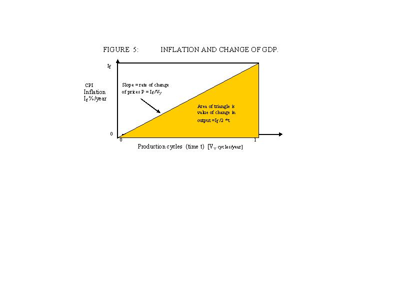
The need to “average” price P can also be shown diagrammatically, as in Figure 5., where the
increase in nominal GDP is the increase in the monetary value of economic output
over a period of time whereas the CPI is the (arbitrarily determined) price level
at any given time. In Figure 5 the GDP value of
the price change If%/year over time t is the area If*t/2,
so that:
% GDP value change = If*t/2 (15)
A CPI
consumer price inflation rate of 2% over time represents a1% inflation in the
aggregate value of goods and services produced during that time, not
2% as is universally assumed. The standard practice of subtracting a percentage rate of CPI inflation from
the nominal growth in the value of GDP output over any given period is therefore
incorrect.
[Figure 5 :
Inflation and change of GDP.]
Even when prices P are arbitrarily
constrained, much greater changes in GDP would be possible if aggregate
incomes were allowed to rise (such as by getting unemployed workers back to work).
The failure to increase incomes proportionately to output is ideological. If
P=1.05 and Vy = 10 as in the example above and production Q is increased to
1500, then:
P =
(My + dMy/dt) / (Q + dQ/dt) *Vy (14)
1.05 =
(100 + 57.5) /
1500 * 10 averaged
Prices P remain the same but there
is a 36% increase in incomes (42/115.5) and a 36% increase (400/1100). There is
no reason why economic output cannot be increased to make use of all the available
economic resources without causing systemic
inflation as long as deposit interest is close to zero and the money supply
increases in proportion to output.
Austerity policies around the world
have failed so dismally because they have arbitrarily suppressed aggregate
incomes, leading to the decay of accumulated non-inflationary growth shown in Figure 4.
MEASUREMENT OF PRODUCTIVITY.
True productivity increases, which
are not typically accompanied by an increase in the money supply, can worsen the measured economic output
because they reduce prices. They are deflationary. Inflation, on the other
hand, increases prices P and the money supply M, not the amount of goods
Q.
There can be no increase in Q unless
there is more production. If the given total work hours and productivity
remain the same, Q must be the same whatever the price level may be. For Q to
increase there must be either more work hours or plant (more labour or capital)
and/or an increase in productivity (more goods and services produced with the
same number of work hours and capital input).
Applying the Fisher equation, a productivity
increase of 10% without an increase in the money supply will cause a fall of
9% in prices:
P =
M / Q *
V
P = ((My + dMy/dt) / (Q + dQ/dt)) * Vy (14)
0.909 = (100 +0) / (1000 +100) * 10 (productivity)
An increase in production resulting
from a population increase of 10% adds 100 to the rate at which output Q is
being produced. To avoid inflation and keep P=1, the money supply would have to
be increased by 10% to 110 because the production increase is monetised (unlike
the productivity gain above which is not monetised) :
P =
((My+ dMy/dt)
/ (Q + dQ/dt)) * Vy (14)
1.0 =
(100+10) / (1000+ 100) * 10
(production)
Suppose now the population increases
by 10% at constant work hours per person and there is also a 10% rise in productivity.
Adding the concurrent effects of
both the 10% productivity increase and the extra production from the 10%
population increase gives:
P = ((My
+ dMy/dt) /(Q +
dQ/dt)) * Vy (14)
0.909 =
(100 +0) / (1000 +100) * 10 (10% productivity)
1.0 = (100+10) / (1000+ 100) * 10 (10% population)
Solving the combined effects of the
10% productivity gain plus the10% increase in production resulting from
population change for price P:
P = ((My + dMy/dt) /(Q + dQ/dt)) *Vy (14)
P =
(100+0+10) /(1000
+100+100) * 10
0.917
= 110 / 1200 * 10
While increases in monetised production
are nominally isolated by measuring GDP output and prices P, as previously
discussed, real productivity increases are not automatically measured in
official output statistics because they are usually masked by price reductions.
In the case of the 10% productivity
increase on its own in the above example, the price level is 9.1% lower [(1-0.909)*100].
When the increased productivity is combined with the concurrent increase in
monetised production due to the 10% population increase, the price level P is
still 8.3% lower [(1-0.917)*100] than it was before the two increases occurred.
To maintain prices P=1.00 with a productivity increase of 10% and a concurrent
population increase of 10% the money supply would have to be increased from 110
to 120 as shown below.
P = (My + dMy/dt) / (Q + dQ/dt) * Vy (14)
1.00 = 120 / 1200 * 10
Orthodox
measurements of GDP and “productivity” fail to reflect real increases in
productivity contributions to output Q. They also miscalculate the measured
monetised growth, as previously discussed. GDP measures the combined PQ side of
the original Fisher equation while disregarding the MV side of the equation.
Using half the Fisher equation for measurement purposes is mathematically
insupportable.
Orthodox methodology determines the
price level P by surveys of consumer prices that are then weighted to produce a
hypothetical average consumer price called the Consumer Price Index (CPI),
which is then used to indicate the price level P contributing to the GDP (PQ).
In orthodox economics and the system
of national accounts (SNA), productivity is typically measured as the increase
of total output PQ for each unit of input (capital and labour), not the
increase of production Q itself, even though the physical increase in production
in many sectors is known and could be used as the basis for accurate
measurement. For example, the primary industries, manufacturing, tourism, but not,
in general, service industries and government, despite attempts to measure
quantitative outputs. The definition and methodology of “productivity” measurement can be found for
This fatal mistake dramatically
affects the entire system of national accounts and the measurement of economic
success in the world economy.
According to the relevant
“productivity” statistics for
If measured “productivity”
PQ/hour rises by 2% and measured price inflation P is, say, 2%, the effect of
that inflation in P of 2% has to be deducted from the real productivity
increase discussed above. The calculation below shows there would then be an
“inflation- free” productivity increase in Q of 0% instead of 2%. Using the
Fisher Equation, the 2% measured “productivity” increase in the rate
of output PQ is really made up of 2% inflation and 0% productivity
gain.
In that case:
P% = My% /Q%*Vy (Vy is held constant at 1.0) (10)
1.00 =
1.00/1.00 * 1.0 (the effect of a 0% productivity gain)
1.02 = 1.02/1.00 * 1.0
(plus the effect of 2% inflation)
1.02 =
1.02/1.00 * 1.0 (total P%*Q% from both effects = 1.02)
Defining productivity
increases in PQ/hour does not necessarily create real increases in output Q.
Assuming they do so automatically is nothing less than wish fulfilment. The
whole concept of improving productivity is increasing Q/unit input (labour and
capital), not the total output PQ.
In practice, CPI inflation in
The measured “productivity”
increase in the example below is a myth.
Using the Fisher equation (10)
again to illustrate the above example:
P% = My %/ Q% * Vy (Vy is held constant at 1.0)
1.02 =
1.02/1.00 * 1.0 (the effect of 2% inflation)
1.00 =
0.99/0.99 * 1.0 (plus the effect of a -1% productivity gain)
1.02 =
1.01/0.99 * 1.0 (total P%*Q% from both effects = 1.01)
Aggregate
changes in production Q can be assessed when output PQ and the price level P
are both known, but productivity changes can only be assessed using both sides
of the Fisher Equation of exchange.
The
relationship between the author’s debt model, inflation and GDP.
As set out in the author’s
papers referred to in this article, the payment of interest on debt in the
debt-based financial system creates systemic
inflation that forces up the productive transaction account money supply My.
In the debt system, if My did not rise, the financial system would
collapse because incomes in the productive sector are continually being
transferred from income earners to deposit holders. The immediate effect is to
reduce the purchasing power of income earners so they literally cannot buy the
goods and services they have produced. Hypothetically,
deposit holders (“savers”) could buy the excess goods and services but that
doesn’t happen because of the “incentive to save” referred to earlier in the
article and because “savers” alone cannot physically absorb the surplus. Instead, in
aggregate, households and businesses are forced to take on the new Ms
debt, which is the systemic inflation arising from net after tax deposit
interest paid on the Domestic Credit (DC) plus
interest paid on secondary debt NBLI, (Nb). The additional servicing
of that additional debt load Ms is a primary cause of increasing
income inequality around the world. In practice, if Ms in the debt
model (equation 3) increases at 4%/year the money supply My in
the productive transaction accounts must also increase by at least 4% assuming
speed of circulation Vy and price level P remain constant as shown
in the examples above.
Equation (9) on page 9 tells a
big story. Stripping out foreign debt and the bubble D b (that is,
in the special case where Dnfca and Mb are both zero),
for the reasons set out on page 9:
[GDP] =
Ms + Dni + R (9)
In the special case of
equation (9), if Ms did not grow, nominal GDP growth would be
largely determined by the monetised value of non-inflationary growth Dni.
For the change in Ms to be zero, deposit interest rates must also be
zero. Since, as already explained above, that is not possible, there will
always be some increase in Ms and therefore some systemic inflation.
That applies whether the financial system is based on bank debt or on Savings
and Loan (S&L) debt.
The main difference between
bank debt and S&L debt is that in the latter case the bank Residual (R)
does not grow as quickly. The innermost secret of the debt-based capitalist
system is laid bare for all to see.
The
net unearned interest income Ms is a fundamental baseline of nominal
GDP growth as shown on Figure 2. Adding less than Ms to the credit aggregate
DCm must contract the measured economy.
Excess
non-productive debt produces excess deposits that typically increase M3 and
systemic inflation as well as inflating non-productive investment sector
prices. As shown above, additional debt-free cash-based purchasing power
introduced to the productive system over and above systemic inflation produces
real growth as long as there are sufficient available human, natural and
physical resources available to the productive economy. That growth is generated
by more hours worked, such as by increases in the working population, reduction
in unemployment, and longer working hours, while the additional contribution of improved productivity can be best
measured by physically measuring the physical quantity of Q/hour, not PQ/hour.
Within the framework of a
capitalist system any monetary reform proposal must introduce more
money into the system (even if it is introduced debt-free) before monetised
“growth” as it is currently measured can occur and, in the relative
absence of traditional bank loans, most of that new money must be on-loaned at
interest through S&L interest-bearing accounts to fund the investment
sector. In the various monetary reform proposals the interest paid on the
S&L accounts will still generate an exponential growth in Ms and
some systemic inflation. Both could, in theory, turn out to be greater than
they are today unless they are carefully managed.
It is
impossible to “produce” a higher GDP (PQ). It is only possible to produce more
(or fewer) goods and services Q. Too much new money Mv will create
inflation. Too little money will induce systemic collapse. The balance in the
productive sector is sensitive because the dynamic productive transaction
account balance Mv is just a few percent of GDP. My
presently circulates (at least in New
The
debt model (equation (3), Figure 2) provides an extremely simple way to match systemic
inflation and non-inflationary growth with extra output enabling GDP to be
increased at near-constant prices.
The difference between
systemic inflation and measured CPI inflation in the present financial system
reflects on-going suppression of wages and incomes. Governments have suppressed
economic “growth” because inappropriate orthodox inflation targeting in the
presence of systemic inflation Ms has meant that incomes have been
unable to grow fast enough to absorb existing output let alone increased
potential output. With the single exception of 1995, systemic inflation in
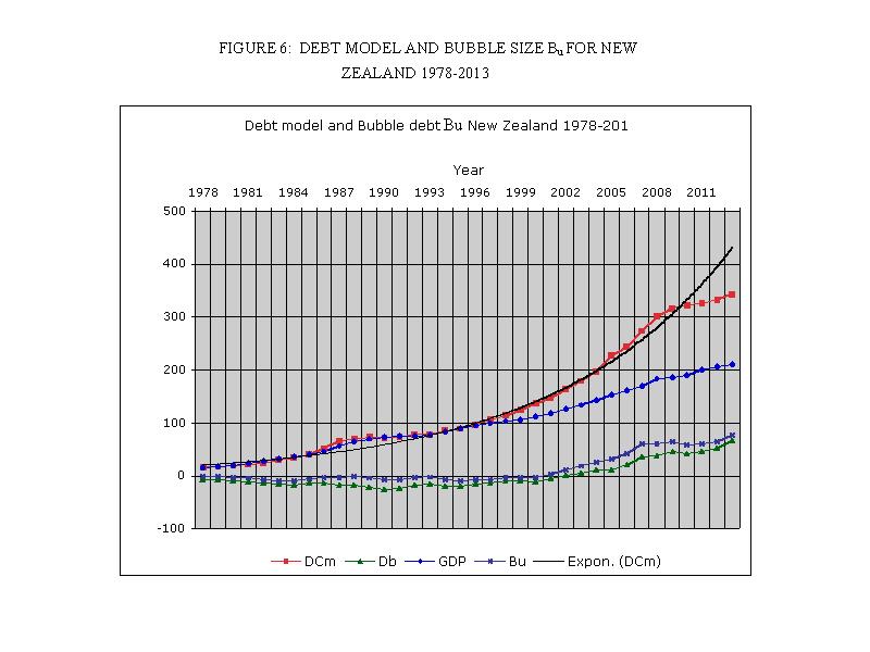
Figure 6 shows the debt model
(Figure 2) solved to obtain a preliminary estimate of the bubble debt Db
in equation (5) for
M3 = [Dmy+ Ms +Dni
+ Db] (5)
Figure
6 shows that orthodox monetary policy bears little relationship to the
mechanics of the debt-based economy. The non-bank debt Nb has to be
added to the bubble debt Db to get the bubble value Bu in
Figure 6 because Figure 6 is based on the total debt
DCm whereas Db is derived from the equation for DC. There
are discernable (quantifiable) bubbles relative to the trend curve of Bu
in
Bubble value Bu
= Db
+ Nb (16)
On
the basis of the preliminary analysis in Figure 6 the 2009 bubble Bu does not appear to have unwound and M3
growth is out of control. That means the Reserve Bank of New Zealand is right
to be concerned about rising prices in the investment sector in New Zealand
because they too appear to be out of control.
The exponential rise in
systemic inflation Ms is inexorable.
It is unlikely that the 2005-2009 debt bubble in
[Figure
6 : Debt Model and Bubble Size Bu for New
Zealand, 1978-2013.]
The bubble debt has been calculated from equation (5) as Db=
M3-(Dmy + Ms+Dni). The separation of (Dni + Db) into Dni
and Db needs further research. For Figure 6 it has been
obtained as the difference between the measured nominal GDP increase and the
change in (Ms+R).
The role commercial banks play
in the capture of GDP has never before been revealed. The banks capture economic growth from the
community at large as shown on Figure 4. Hence equation (9):
[GDP] = Ms + Dni + R (9)
Where:
Ms = Systemic inflation
Dni =
Non-inflationary growth
R = Bank residual captured from GDP.
Figures 4 and 6 indicate that
unless the exponential growth of the model systemic inflation (Ms)
is halted, the
CONCLUSION.
This paper hints that the
Exponential debt-growth and
productive sector inflation are synonymous with capitalism. This point is
discussed at length in the author’s paper Capital is Debt.
Governments and economic policy
makers have striven to make square policy pegs fit round economic holes
subjecting the world and its people to boom and bust cycles with immeasurable
consequences.
This paper suggests that sound
monetary management can produce dramatically better economic outcomes
worldwide. To do so will mean abandoning the myths about inflation, growth, and
monetary mechanics that underpin orthodox macroeconomic policy and at the same
time fail to satisfy the basic accounting equation.
Abandoning those myths will mean:
-
strictly managing cross border capital flows using
powerful tools such as a Foreign Transactions Surcharge.
-
using the revised Fisher equation of exchange
(equation (3) outlined in this paper (or similar) to enable the money supply to
be properly aligned with potential economic output.
-
introducing broad monetary reform such as the Manning Plan (or similar) to keep
interest rates as close to zero as possible.
-
constraining secondary debt growth as the use of
interest-bearing bank debt is phased out in the course of implementing monetary
reform proposals.
-
ensuring that the macroeconomic model chosen satisfies
the basic accounting equation at all times.
-
abandoning the methodological fallacies in the
calculation and use of the CPI inflation index and GDP calculations.
-
introducing a valid methodology to measure and account
for true increases in productivity and/or production.
Bubbles occur in the investment sector due to uncontrolled debt growth Db
while, at the same time, the productive sector is suppressed through arbitrary
orthodox macroeconomic policy settings. The debt bubbles have occurred because
of fundamental misconceptions about the way the financial system works.
Lowell Manning,
Wellington,
07 July, 2013.
Summaries of monetary reform
papers by L.F. Manning published at http://www.integrateddevelopment.org.
Chicago Plan Revisited Version II: An insufficient
response to financial system failure. (Posted 11 May, 2013.)
Comments on the IMF (Benes and Kumhof) paper “The
Chicago Plan Revisited”.
Debt bubbles cannot be popped : Business cycles are policy inventions.
DNA of the debt-based economy.
General summary of all papers
published.(Revised
edition).
How to create stable financial systems in four
complementary steps. (Revised edition).
How to introduce an e-money financed virtual minimum wage
system in New Zealand. (Revised edition) .
How
to introduce a guaranteed minimum income in New Zealand. (Revised edition).
Interest-bearing debt system and its economic impacts.
(Revised edition).
Manifesto of 95 principles of the debt-based economy.
The Manning plan for permanent debt reduction in the national economy.
Measuring Nothing on the Road to Nowhere.
Missing links between growth, saving, deposits and
GDP.
Savings Myth. (Revised edition).
Unified text of the manifesto of the debt-based
economy.
Using a foreign transactions surcharge (FTS) to manage the
exchange rate.
(The
following items have not been revised. They show the historic development of
the work. )
Financial system mechanics explained for the first time. “The Ripple
Starts Here.”
Short summary of the paper The Ripple Starts Here.
Financial system mechanics: Power-point presentation.
"Money
is not the key that opens the gates of the market but the bolt that bars
them."
Gesell,
Silvio, The Natural Economic Order, revised English edition, Peter Owen,
![]()
This work is
licensed under a Creative
Commons Attribution-Non-commercial-Share Alike 3.0 Licence.