NGO Another Way (Stichting Bakens Verzet), 1018 AM Amsterdam, Netherlands.

SELF-FINANCING, ECOLOGICAL, SUSTAINABLE, LOCAL INTEGRATED DEVELOPMENT PROJECTS

FOR THE WORLD’S POOR.

Homepage	Projects, examples	WRITE AN INTEGRATED DEVELOPMENT PROJECT	FREE E-COURSE FOR DIPLOMA IN INTEGRATED DEVELOPMENT	Articles and resources	About Us
Downloads (updated 03 October 2011)	More on development issues			Some useful technologies	Contact us

Edition 01 : 23 October, 2014.

( FRANÇAIS)

HOW THE WORLD’S POOR CAN IMPROVE THEIR QUALITY OF LIFE AND MEET THE MILLENNIUM DEVELOPMENT GOALS.

PRACTICAL MONETARY REFORM.

(Stichting Bakens Verzet has endorsed the Earth Charter.)

Return to : Stichting Bakens Verzet Homepage.

BEYOND PIKETTY: THE ANATOMY OF INEQUALITY

By Lowell Manning

manning@kapiti.co.nz

Sustento Institute Christchurch

www.sustento.org.nz

Version 4: 22 October 2014

CONTENTS.

1. Executive Summary.

2. Introduction.

3. The “Golden Rule” and the Fundamental Laws”

4. Verifying Piketty’s “first law”.

5. Verifying Piketty’s “second law”.

6. Reconciliation of growth, saving and inflation.

7. What is “capital”?

8. Inequality and bubbles

9. Conclusions.

10. References.

Acknowledgement:

The author acknowledges the invaluable input and editing by Terry Manning, NGO Bakens Verzet Holland www.integrateddevelopment.org

1. EXECUTIVE SUMMARY

This paper establishes the source of inequality using Thomas Piketty’s recent book “Capital in the Twenty-First Century” as a reference point.

Saving as measured in each country’s national accounts has a growth component and an inflation component.

The source of systemic inequality is the inflation component of Saving plus bubble debt.

Systemic inequality is defined by a set of 8 macroeconomic accounting principles:

1. The present (reflated) value of all past real growth ∑g_r is the Gross Domestic Product, GDP.

2. The present (reflated) value of all past saving ∑s_r is the produced tangible wealth as measured in each country’s national accounts.

3. In the absence of bubble debt the present (reflated) value of inflation, ∑s_r - ∑g_r is the accumulated systemic inequality built into the capitalist financial system.

4. The value of total wealth is the present value of all past saving imputed by market transactions to include intangible and non-produced wealth.

5. The sum of existing (non-reflated) outstanding productive investment principal ∑P is the Gross Domestic Product GDP.

6. Outstanding investment productive principal ∑P = the present reflated value of all past real growth ∑g_r = GDP.

7. In the absence of Quantitative Easing and other bubble debt the systemic increase in inequality which can be defined as the growth of the unproductive investment sector relative to the productive sector, will stop when (saving “s” = real growth “g”); that is, when systemic inflation which can be defined as the after-tax deposit interest paid on the country’s total bank deposits, is zero.

8. Using Piketty’s terms, numerical inequality will decrease only when the rate of return “r” on the national capital falls below the real economic growth rate “g” divided by the ratio “β” of national capital (national wealth) to national income.

Inequality is endemic to capitalism and debt-based economies.

Wealth is transferred upward through the deposit interest rate mechanism whereby the net interest paid by original debt holders under their debt contracts finds it way as unearned income to current deposit holders’ accounts. That unearned income is funded from nominal GDP growth and confers higher values on all traded national capital, not just its income producing portion. That is what increases inequality.

Reversing that structural inequality under the present system requires (r<g/β), or, in simple terms, that capital “runs at a loss” even when deposit interest is zero. The capital (wealth) base would then gradually deflate without affecting economic growth. This would not be capitalism as it is presently practised because new wealth would then tend to be distributed according to earned income.

Housing remains a core issue within the capitalist system worldwide because most domestic housing is economically unproductive. Its capital cost can only be repaid over time out of increased productivity passed on to income earners. Each expensive new house built means part of a factory or farm or other productive enterprise might be lost. Building expensive houses instead of cheaper ones has produced a wealthy over-housed minority and a poor under-housed majority. The same argument applies to public infrastructure, services and transfers.

The tax reforms Piketty proposes in Part Four of his book would reduce inequality much as happened when the “U” shaped wealth profiles were formed in some countries during the 20th century (as shown at Figure 4.5 of his book). The reforms did not prevent the revival of capital inequality as their effects were whittled away over time. The reforms failed because the crucial roles credit creation and public policy play in income and wealth distribution have been neglected in recent decades.

Rising structural inequality suggests that the financial system itself needs to be modernised. There are several viable options available, including combinations of “bottom up” local currency proposals where the local currency can be used to pay taxes, “top down” approaches based on interest-free public money, and much broader use of cooperative economic activity.

This paper also shows that the “fundamental laws” Piketty proposes in his book do not withstand scrutiny. There is no causal link between income and wealth inequality measured by Piketty’s ratios (β= national capital/national income) and his two productive sector ratios, (β= s/g (savings/accumulated growth)) and (β = α/r), where “α” = the ratio of annual capital income to annual national income” and “r” = the annual rate of return on capital.

2. INTRODUCTION

Piketty’s book “Capital in the Twenty-first Century” is primarily a study of inequality. The heart of his book and his “laws” (as further defined below) is that the percentage (r-g) gives rise to a capital-based unearned income that is surplus to the monetary requirements of the productive economy.

The equations from Piketty’s book are applied to official economic statistics for Australia and New Zealand.

Piketty’s own data set for Australia shows his “laws” to be false.

“Capital in the Twenty-First Century” is founded on three concepts. These are:

1) A so-called “golden rule” (r>g) where “r” is the percentage (%) annual rate of return on capital (national wealth net of debt, as Piketty defines it) [p50] and “g” is the real growth rate of annual economic output (Piketty uses National Income instead of Gross Domestic Product GDP) as measured by the international System of National Accounts (SNA).

2) A “First Fundamental Law of Capitalism” (α= r x β) where alpha “α” is the ratio of annual capital income to annual national income given as a percentage, “r” is the percentage annual rate of return on capital, beta “β” is the ratio of national capital (national wealth, as Piketty defines it) to national income [p52].

3) A “Second Fundamental Law of Capitalism” (β= s/g) where beta “β” is as already defined, “g” is the accumulated “long run” annual real growth, (apparently stated as an annual percentage), and “s” is the accumulated “long run” savings which appears to be the “ net savings rate” derived from the national accounts (also apparently stated as an annual percentage) [p166].

A) Referring to Piketty’s indicator (β= s/g) (as defined above):

The long-term productive sector ratio (s/g) for New Zealand from 1962-2013 is shown in Figure 10. Figure 10 demonstrates that for New Zealand in 2013 (by way of example) when the estimated ratio of national capital/national income, “β”, was about 6, (s/g) was just 3.2. Contrary to Piketty’s assertions that the value of “β” results from long term trends, Figure 10 shows that “β” calculated as (s/g) is volatile over the short term (Figure 10, for the period 1977-1995) when the divisor “g” approaches zero.

The paper shows that Piketty’s ratio (s/g) is a measure that reflects the relationship between prices and output in the productive economy. Asset prices are defined by the aggregate physical transfer of Saving “s” from the productive economy to the non-productive investment sector as shown in Figures 2,4,7,and 13.

B) Using Piketty’s indicator (β = α/r) (as already defined above):

In Figure 8, the annual rate of return on capital “r” from Piketty’s equation (r=α*g/s) is compared with an actual estimated rate of return on capital for New Zealand for the period from 1978 to 2012.

The result shown in Figure 8 suggests there is little or no relationship between the calculated annual rate of return on capital using Piketty’s equation and the actual rate of return for New Zealand. For simplicity, a constant figure for “α” of 30% (as proposed by Piketty in his book, although he actually uses after tax figures in his data set that are only about half that) was used when evaluating the Piketty equation. The validity of the equation (r=α*g/s) was tested for New Zealand for 2012 (α =27%) and for 1988 (α =35%). Using after-tax figures for “α” changes its position on Figure 8 but not its shape.

3. THE “GOLDEN RULE” AND THE “FUNDAMENTAL LAWS”

“The Golden Rule”

Piketty says the “Golden Rule” (r>g) is “the central thesis of this book” [p77] because “an apparently small gap between the return on capital and the rate of growth can in the long run have powerful and destabilizing effects on the structure and dynamics of social inequality”.

Piketty neglects debt (and money) in his book altogether except during a brief discussion on public debt (pp. 547-552). That neglect is fatal to his thesis.

Plainly, Pikkety’s “net” investment return (r – g), applied to market activity in the productive sector, will inflate asset prices if it is positive. It will do so because “r”, the annual percentage (%) rate of return on net national wealth as Piketty defines it [p50] on the one hand, and “g”, the annual real growth rate of economic output (Gross Domestic Product or GDP- Piketty uses National Income-) as measured by the international System of National Accounts (SNA) on the other, both give rise to exponential functions over time. For example, if “r” were 7%/year, $1000 of wealth would increase to $2000 over 10 years. If on the other hand “g” were 3.5%/year, it would take 20 years for $1000 of “g” to increase to $2000. The historical “r” and “g” curves will therefore diverge rapidly. That divergence is the primary indicator of growing inequality.

This paper shows in detail that the only way to avoid asset price rises in the capitalist system is for the numerical after-tax rate of return on capital to be well below the real economic growth rate “g”. That, however, is the antithesis of capitalism. Asset inflation and exponential wealth expansion are therefore inherent in the capitalist system unless capital (money) is physically destroyed for example by bank failures, as happened during the great depression of the 1930’s.

When “r” is greater than “g” (r>g) the financial system is subject to inflation and investors may typically be able to accumulate surplus deposits over and above those resulting from economic growth. Piketty does not tell us how the increase in investment sector deposits creates the redistribution of wealth to investors from the rest of society but his “golden rule” is a good indicator a transfer is happening.

Describing how the transfer actually takes place calls for an understanding of the dynamics of debt-based financial structures and of “saving”.

The saving “s” Piketty uses is the “net saving” from the national accounts using the System of National Accounts (SNA). It is supposed, according to Piketty, to fund the net increase in physical capital assets at cost resulting from the growth of economic output (Gross Domestic Product or GDP). This paper shows that the aggregate saving “s” in the national accounts is less than the aggregate nominal GDP growth because the national accounts wrongly deduct consumption of fixed capital from gross capital formation whereas the actual financial flows, being the repayments of principal on outstanding productive sector debt, should instead be used.

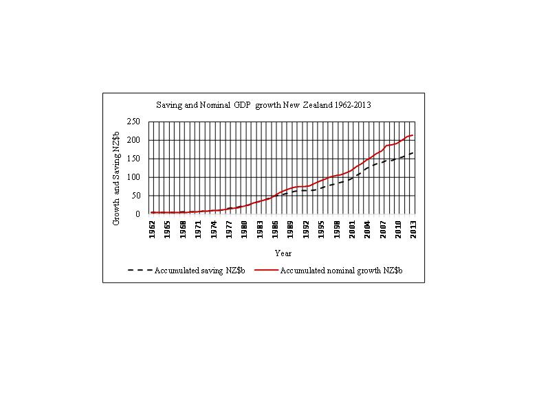
The expressions (r-g) and the “golden rule” (r>g) ultimately refer to inflation although Piketty does not seem to be aware that is so. Figure 1 shows the actual accumulated numerical figures ∑s for saving “s” and ∑g for real growth “g” for New Zealand. Using Piketty’s typical figures, the separation between the two curves will be different in other countries but they will have the same shape.

The inflation transfer mechanism makes the curves for “s” and “g” in Figure 1 diverge.

Figure 1. Accumulated “s” and real GDP growth “g” New Zealand 1962-2013.

Piketty’s “First Fundamental Law of Capitalism” (α= r x β)

Piketty himself says the “first law” is a tautology (p52). (Capital Income/ National Income = r * net national wealth / National Income) says (Capital income = r * net national capital (wealth)) because the national income cancels out from each side of the equation.

The “first law” states that income from capital is the [capital base (net national capital or wealth as Piketty defines it)* the average annual rate of return “r” (or “yield”, p52, on that wealth.)] The “first law” fails to link the productive economy properly to the investment sector even though productive sector incomes must be used to physically pay the capital income represented by “r”. The non-productive investment sector does not produce anything itself and Piketty (p45) makes abundantly clear that rentiers historically didn’t work and that their (unearned) income came from their ownership of wealth.

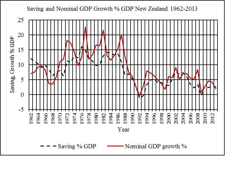
Figure 2 shows measured national account SNA “Saving” “s” plotted against nominal percentage GDP growth for New Zealand over the past half century. (Figure 4 shows what happens when real GDP growth figures are used instead).

Figure 3 shows the same for Australia. Net interest after tax paid from work income is transformed into capital through productive sector inflation. The resulting shortage of purchasing power in the productive economy caused by the withdrawal of that capital income can only be filled by new debt.

That new debt causes the inflation that creates the wealth inequality seen around the world.

Figure 2. Saving and Nominal GDP Growth as % GDP New Zealand 1962-2013.

Figure 4 shows the accumulated data for nominal GDP growth and saving “s” from Figure 2 for New Zealand. The saving and GDP curves are much closer together there than they are in Figure 1 because nominal GDP growth has been used in Figure 4 instead of real GDP growth as shown in Figure 1. The accumulated Saving curve in Figure 4 is still below the real accumulated nominal growth curve because consumption expenditure in the national accounts incorrectly includes the difference between physical capital repayment flows and depreciation (consumption of fixed capital). [GDP, gross capital formation, consumption of fixed capital and saving all need to be higher as discussed in Section 5 of this paper.]

Figure 3. Saving and Nominal GDP Growth as % GDP Australia 1962- 2011.

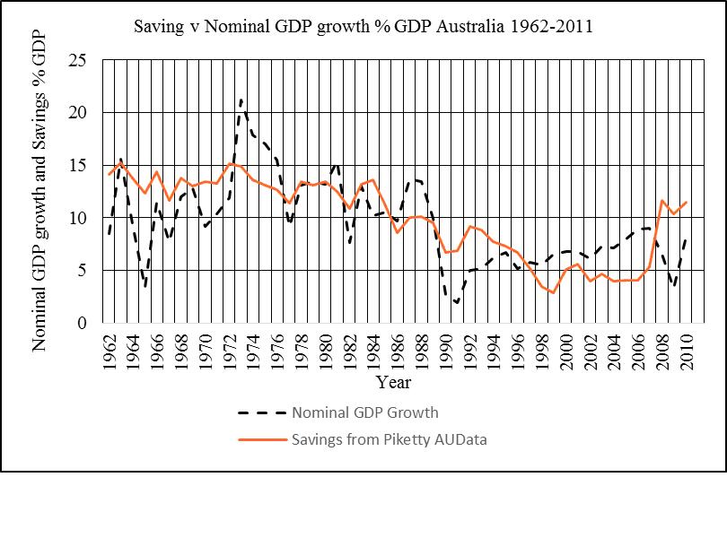
Source: Piketty Zucman dataset

Figure 4. Accumulated Saving and nominal GDP growth : New Zealand 1962-2013.

Source: New Zealand National Accounts

When the Saving figure as shown in Figure 2 is (arbitrarily) corrected for New Zealand by about 23% to cover the difference between the (higher) physical capital repayment flows and the (lower) rate of depreciation (consumption of fixed capital) used in the SNA accounting system, the GDP and outstanding investment principal curves fall on top of each other as is shown conclusively in Figure 5 for New Zealand.

GDP is therefore the sum of outstanding investment principal.

Figure 5. Outstanding investment principal v GDP New Zealand 1962-2010.

Sources:

The Savings Myth (http://www.integrateddevelopment.org/lowellsavingsmyth20110522.htm ;

The DNA of the debt-based economy http://www.integrateddevelopment.org/lowellDNApaper20110805.htm

An independent test for “r” is to compare the figures for (r_dt = α_dt/β) derived from the “first law” in Piketty’s (Piketty-Zucman data) Table 3b with the formula (r_dt = α_dt* g/s) which is derived as discussed below. The “saving” in the productive sector that funds non-productive investment relates directly to the growth of productive sector debt required to fund the net after-tax interest on the country’s deposit base. [Manning 2011a, Manning 2013a]. This means that while (r>g) may indeed be an indicator of divergence between net national capital and national income it cannot numerically define it. This is shown beyond doubt in Figure 7 below.

Piketty’s “Second Fundamental Law of Capitalism” (β= s/g)

Piketty discusses his “Second Fundamental Law of Capitalism at some length [pp 168-176]. The second “law” says that (β= s/g) where beta “β” and “g” are as already defined and “s” is the “savings” (net after tax) from the national accounts [p166].

Piketty’s effort to link the productive economy to wealth as he defines it is confused. For Piketty, national wealth includes the “stock” of the current monetary value of every investment asset, and he lists those at several points. He divides them into farmland + housing + other domestic capital (both private and public) +net foreign capital. At page 47, Piketty says natural resources such as “petroleum, gas, rare earth elements, and the like” are included in that capital, but he does not focus on the difference between the wealth itself (the assets) and the monetary “value” given to those assets.

He further confuses his definition of wealth when he writes [p196] that “By definition, the law (β= s/g) applies only to those forms of capital that can be accumulated. It does not take account of the value of pure natural resources, including “pure land …”.

Farmland is apparently not “pure land” “prior to any human improvements.”

As discussed below for New Zealand, net national capital (wealth) as defined by Piketty cannot be directly represented by the national saving figures nor even by the capital stock given in the national accounts. That capital stock is only about half of all national wealth in New Zealand. Many items like the natural resources Piketty includes in his definition of net national capital are specifically excluded from the capital stock in the SNA system of national accounts.

Piketty defines the annual rate of return on capital or yield “r” as a net % return “over the course of a year” [p52]. His dataset for Australia [Piketty-Zucman Wealth-Income data Set Australia – Table 3b] derives “r_dt” from the net after-tax capital share in National Income, “α_dt”, by using his estimate for “β”. That does not give a verification for “r”. A rate of return can be paid only on the market portion of national wealth that is funded by the productive economy. It is not paid on unrented wealth like the commons, the public estate, owner occupied property, valuables, non-commercial vehicles or even on inventory.

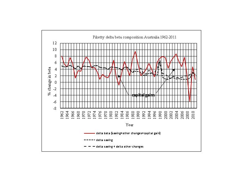
Although Piketty talks about his second “law” (β= s/g) throughout his book, his own work shows it to be false. His Table 5a [Piketty-Zucman Wealth-Income data Set Australia] states categorically that changes in “β” are made up by adding three elements: the “savings induced wealth growth” (g_wst =S_t-1/B_t-1), other volume changes (O_t =O_yt/β_t) and the “real rate of capital gains” “q_t”. For the year 2000 for example, “∆β” was 7.5%. The Piketty-Zucman calculation is given as:

∆β 7.5% = 0.3% (g_wst from saving) + 1.4% (O_t ) + 5.9% (q_t ).

In other words, almost none of the change in “β” in Australia in the year 2000 came from savings even according to Piketty himself. Figure 6 gives Piketty’s own data (from the same Table 5a) plotted for Australia. Figure 6 shows there is no relationship between “β” and saving “s” let alone for saving/growth (s/g).

Piketty claims his “second fundamental law” has to be applied over the long term. Figure 7 shows “β” from Figure 6, the growth in “β” from savings “g_wst” from Figure 6 and accumulated “s_t/gt” also from Figure 6 accumulated over a half century.

Figures 6 and 7 use Piketty’s own data. They confirm the work of the author of this paper and show that Piketty’s own “laws” are wrong.

Figure 7 shows the changes in “β” are related to savings “s_t” not to the change in savings/growth (s_t/g_t).

Allowing for the issues already discussed for New Zealand relating to the failure to use actual principal repayments in the national accounts, saving “s” is proportional to the increase in wealth, not equal to it. Figure 5 shows total accumulated outstanding investment in New Zealand’s productive sector. Percentagewise, Figure 7 for Australia (which starts with Piketty’s value for “β” in 1962) mirrors Figure 5 for New Zealand.

In aggregate people have to “save” some of their income even in the absence of growth to pay for the “hand held out at the market gate” [Manning 2013b]. That seems to have happened in New Zealand in the high inflation period of the 1970’s and 1980’s as shown by the peaks in Figure 2 and by the saving and growth figures in the national accounts. Income is transferred from interest-paying debtors to interest-collecting deposit holders and becomes part of the capital income “Saving” “s” recorded in the national accounts.

Figure 6. Composition of ∆β - Australia 1962-2011 (Piketty Table 5a).

Figure 7. Piketty’s % increase in “β” related to % increase in Saving and % increase in Saving/Growth- Australia. 1962-2011.

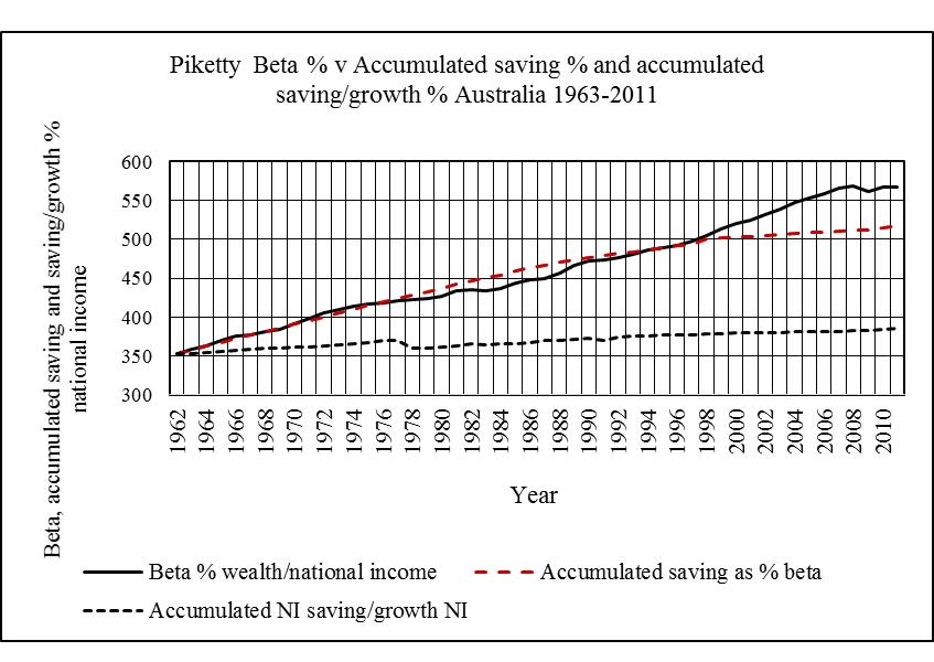
In a debt-based system, central bank policy to manage inflation by raising interest rates reduces the demand for new debt (because the price of debt rises) while at the same time transferring more purchasing power from consumption in the productive sector to the investment sector through systemic inflation [Manning 2011a].

Existing asset prices rise only until investors withdraw from active non-productive investment as the passive interest return on deposits increases. At that point the price of investment assets falls and debt cancellation through physical repayment, business failure and household default begins. Changing interest rates have a similar effect on investment markets as major world events do: they cause a shift in the mix of active investment in relation to properties, equities and bonds that can lead to systemic collapse in both the productive and investment sectors.

The resulting additional SNA “saving”, part of “s”, accruing from the higher interest rates is dissipated in inflation in both the productive and the investment sectors and the consequent reduction of consumer demand and productive investment typically causes an accompanying recession. If that failure were to continue over a lengthy period without new debt creation there would soon be little money left in the productive economy and few productive assets left. That is what happened during the 1930’s depression. To avoid deflation in the productive economy the money supply would have to be increased through higher government spending or some other stimulatory monetary policy as has happened recently around the world through quantitative easing.

Piketty fails to address these financial system mechanics even though they form the basis for establishing asset “values” under his “second law”.

4. VERIFYING THE FIRST LAW

The two “laws” (β=s/g) and (α= r * β) are not truly independent because (from (s/g=a/r) they give other forms like (r=α*g/s).

These derived relationships are at the heart of Piketty’s suggested long term decline in the rate of growth in developed countries though he does not prove them. The decline in the rate of economic “growth” has a far simpler explanation related to the increasing proportion of services in developed economies. It is much harder to increase productivity in services than it was to increase industrial productivity during (say) the industrial revolution, while increases in bureaucratic complexity and compliance costs often lower quality of life instead of improving it.

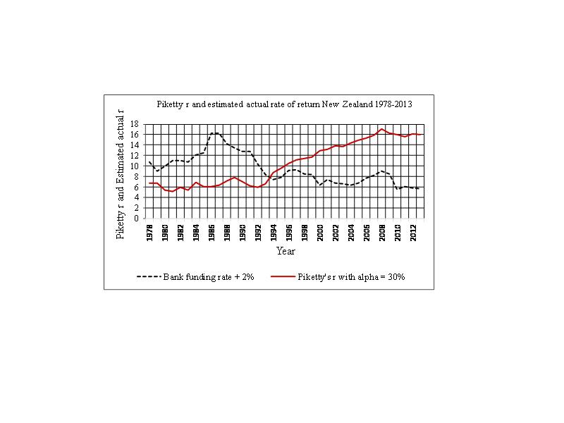
Consider (r=α*g/s) in Figure 8, using “α” = 30% , indicated by Piketty as a typical value for it [p53]. Mathematically, the only time “g” can be 0 is if (r=0) or (s/α =0). However, Piketty is not working “mathematically”, because he considers “s” and “g” to be aggregates accumulated over the long term. Figure 8 shows Piketty’s “r” compared with an actual estimate for it (using the bank funding rate + 2%) calculated from the aggregated dataset for New Zealand for the period 1978-2013. Figure 8 shows that Piketty’s “r” is unrelated to the actual value of “r” in the New Zealand economy over the period 1978-2012.

Figure 8. Piketty’s “r” compared with Actual rate of return, “r”, New Zealand 1978-2013.

Piketty’s “r” in Figure 8 is derived as (r=α*g/s) from the accumulated historical data used in Figure 1 where “α” is the pre-tax figure he refers to throughout his book. The after-tax figure “α_dt” that Piketty calculates in his data set for Australia [Piketty-Zucman Wealth-Income data Set Australia – Table 3b] is about half the pre-tax figure used in Figure 8 and it is reasonably constant through the whole period except 1999-2000 and 2005-2008 (when it was several percent lower). Using after-tax figures in Figure 8 changes the position of the curve but not its shape. The actual rate of return estimated from the bank funding rate is plotted on an annual basis.

The plot for Piketty’s “r” in Figure 8 gives an irrational result. An average rate of return “r” over the entire wealth (net national capital) base of 16% as shown in Figure 8 for New Zealand in 2013 is impossible when mortgage interest rates there were less than half that. In New Zealand’s case, based on its wealth (net national capital) in current dollars of about NZ$ 1200 billion, 16% would be NZ$ 192b or nearly the entire GDP! Even when an after tax figure of, say, half the above value of “α” is used (as Piketty does in his data sets), almost half of New Zealand’s GDP would still be paid to rentiers. The pre-tax figure of 30% for “α” used in Figure 8 has been checked for New Zealand by adding the “market” interest and dividends from Table 2.1 of the national accounts and then adding a derived figure for rent. The “Producer enterprises sector accounts” (Table 2.1) gave a total of NZ$ 44.7b for 2012 for interest and dividends. The author has assessed the “non-market” rental of privately held rental property to be about NZ$ 8b based on a gross rate of return of 7% and a private non-business rental base of NZ$ 115b. That NZ$ 8b added to the capital income from interest and dividends of NZ$ 44.7b (from the New Zealand national accounts for 2012 as above) gives a total gross figure for interest, dividends and rents of about NZ$ 53b.

New Zealand’s gross national income in 2012 was NZ$ 198b, so “α” was then about 53/198 or a little under 27%, close enough as a first approximation to the 30% Piketty considers as a “typical” figure for developed countries. Figure 8 therefore gives a rational representation of Piketty’s “r” (before tax) as long as “α” is reasonably close to 30%.

Piketty’s “α” was also checked for an “extremely” high interest year (1988) when the Gross national income (NI) in New Zealand was NZ$54.5b, total debt was NZ$57b, and the comparable return on capital (from Figure 8) was 14.3%. Assuming similar proportioning of investment returns in 1988 as in other years, the capital income/national income ratio “r” would have been closer to 35% producing a small peak in the Piketty “r” graph as shown on Figure 8 during the 1980’s. This is much too small to affect the conclusion presented above that Piketty’s “r” is unrelated to the actual annual rate of return on capital.

Figure 9 plots the rate of return “r” (after tax) taken directly from Piketty’s data set for Australia [Piketty-Zucman Wealth-Income data Set Australia – Table 3b] over the last half century using Piketty’s two laws independently. The two laws give completely different results proving that at least one of them is false.

5. VERIFYING THE SECOND LAW

Piketty says (p48) that wealth is net of “the total amount of financial liabilities (debt)” and that agrees with the approach taken in the capital stock calculation used by the New Zealand Department of Statistics.

Figure 9. Piketty’s own “r_dt” from (α_dt/β) and (α_dt*g_t/s_t) Australia. 1962-2011

Piketty’s book hinges on the “U” shape in national capital over the period from the start of WW1 to just after WW2 [Book Figures 3.1, 3.2]. He writes that that “U” shape is due almost exclusively to war debt and wartime inflation and the effects of the 1930’s depression. For example, average inflation in France between 1913 and 1950 was 13% (p 545). In Germany the comparable figure was 17% (p 545). Piketty repeatedly says this period was unique in economic history [Ch 4] though New Zealand and many other countries had inflation rates as high or higher in the 1970’s and 1980’s than the ones he quotes. He describes what happened to wealth during his “U” period, but he doesn’t tell us how it happened. Instead, he writes: “[T]he decline in the capital/income ratio between 1913 and 1950 is the history of Europe’s suicide, and in particular the euthanasia of European capitalists” [p 149]. Whatever merit Piketty’s comments may have they are unhelpful to proving his “laws” because Europe has in fact survived very well. Moreover, much of his book is about the revival of European capitalists, so while they may have suffered between 1913 and 1950 they were clearly not “euthanased”.

How the change in wealth came to form Piketty’s “U” is set out below without using either of his “laws”.

The two source papers [Manning 2012, Manning 2013a] suggest that the cumulative outstanding productive investment principal at cost ∑P and the accumulated saving ∑s_t are both numerically equal to nominal GDP as shown in Figures 4 and 5.

Both Piketty’s “s_t” and Saving “s” must be after-tax figures because government spending is already included in “total consumption” in the national accounts. The principal repayments actually paid by firms are physical monetary flows whereas the residual Saving recorded in the national accounts is an accounting abstraction, despite the strenuous efforts made by statistical authorities to generate an appropriate figure for “Consumption of Fixed Capital”. For an example of those efforts see “Measuring Capital Stock in the New Zealand Economy” 3^rd Edition, published by Statistics New Zealand, Wellington, 2013.

Nobody pays anything called “consumption of fixed capital”. Instead, principal is repaid on capital items bought, in addition to interest. The repayments on productive assets must be funded from the gross operating surplus resulting from business activity in the productive sector. Payments of interest and capital relating to non-productive investments like housing must come from the work incomes of income earners: typically from wage increases generated by higher labour productivity.

Capital repayments in the productive sector must be more than the amount shown in the national accounts for the consumption of fixed capital. If that were not so, the banking system would have no residual security over the capital items they have funded as those assets approach the end of their useful life. For example, commercial vehicles have a scheduled life of around 7 years, but are typically paid off over 5 years or less. Residential buildings are allocated a 70 year life cycle, and are frequently paid off over 20 to 30 years. The “Savings” “s” in the SNA accounts, on the other hand, merely reflect post depreciation (amortisation) asset values which comprise tax-based accounting entries. Real residual monetary values are shown by the purchase price less actual repayments.

Once an appropriate correction to the consumption of fixed capital is made for those actual capital repayments, the SNA saving should equal the increase in productive capital (Gross capital formation less capital repayments) at current (typically inflated) prices. That is the basis of the Savings Myth [Manning 2011b]. SNA Saving “s” should be the net new capital creation and that must also equal nominal GDP growth as shown in Figures 4 and 5.

Theoretically at least, the productive economy is a closed circuit of financial flows where real financial surpluses are used to fund gross fixed capital formation at cost (Manning 2013a). That re-investment creates debt, either to the income earners and businesses who have produced the assets or to the banks. The resulting deposits attract interest that contributes to systemic inflation.

Further research is needed to confirm how the additional principal repayments (total principal repayments – consumption of fixed capital) added in Figure 5 to the figure for “consumption of fixed capital” could (or should) be shown in the national accounts. The total principal repayments would be recorded in the national income and outlay account (Table 3.2) where “consumption of fixed capital” is shown now, reducing national disposable income. The gross operating surplus (with GDP and gross fixed capital formation) may therefore be understated in the income and expenditure account of the national accounts (Table 3.1). The residual “Saving” “s” would then consequently increase by the same amount in the national income and outlay account to rebalance the accounts. Otherwise the additional capital repayments would suppress consumption as a percentage of GDP and mask the systemic inflation discussed in the source papers. Masking (from somewhere) seems to be a primary reason the observed CPI inflation as it is customarily reported in statistics is less than the systemic inflation discussed in the source papers. The suggested changes would not affect real economic growth. They would affect nominal reported GDP growth and the way inflation is reported.

The national accounts produced under the System of National Accounts (SNA) are only as accurate as the data on which they are based and the data series are constantly being reviewed. For example, the New Zealand “saving” data was recently amended upwards by up to 2% of GDP to take account of updated estimates of spending by foreign visitors. By comparison, adding about 23% to consumption of fixed capital to account for “actual repayment of principal” would increase “saving” in New Zealand for 2013 by 3.2% of GDP and better reflect systemic inflation.

Quite apart from required amendments to the data used in the national accounts, Saving in the national accounts is independently subject to wide margins of error because it is a small number resulting from subtracting much larger numbers each of which is itself subject to considerable error. That is especially the case when Saving “s” is small.

Compulsory savings and pension schemes add to the “saving” problem because they reduce demand in the productive economy unless all the withdrawal of purchasing power they cause is re-invested in new capital goods. If that re-investment does not occur the withdrawals become part of nominal “saving” that is diverted into investment sector inflation. This is because the hoarded “saving” is either left in bank accounts at interest or is added to the deposits used to trade existing assets in the non-productive sector. Indeed, in the case of New Zealand’s Kiwisaver scheme, fund managers were mostly prohibited from investing in new production, thus guaranteeing a loss of growth in the productive economy and an increase in speculative “investment” expectations.

Since the deposit investment pool (the total financial deposit base less the relatively small amount of deposits used in the physical production of goods and services) follows GDP (after substituting actual repayments for depreciation) [Manning 2012, Manning 2013a] a percentage increase in GDP (Piketty uses national income Y) tends to produce a similar percentage increase in wealth however that wealth is calculated. If the investment pool deposits increase by 10% all investment prices in aggregate, including the prices of non-produced capital, will also increase assuming the proportion of active investment in equities, property and bonds, remains constant. If, on the other hand, investors withdraw from active trading in existing assets thereby increasing the proportion of passive interest-bearing deposits, the circulating pool of active deposits used for investments will fall and so will investment prices. Shifts between the investment categories can also occur with changes in public policy, taxation, or external events.

Investment in the productive economy, as it must do, creates nominal GDP growth derived from multiplying price “P” and production “Q” in the Fisher equation (MV=PQ) where M is the money supply and V is its speed of circulation. It does not separate out inflation. The new debt used to purchase new capital assets determines wealth growth. Figure 7, which refers to Australia, shows that comparing inflation-adjusted growth figures with saving has nothing to do with generating “wealth”. Real growth can be zero or even negative while the non-productive investment sector still expands rapidly if inflation is high, as happened in New Zealand in the 1970’s and 1980’s. The nominal cost of replacing existing assets then increases.

The most extreme case of low growth and high saving in New Zealand was in 1980 when saving “s” was 16% of GDP and economic growth was -1.7%! During the high inflation period the gross operating surplus (and with it gross fixed capital formation) soared while “old dollar” principal repayments were being made in rapidly inflating currency. The high interest rates were bound to produce a very large national account “saving” figure that was obviously not all spent on creating real growth, especially in years like 1980. Instead “s” in those years represented productive sector inflation.

After replacing actual principal repayments for the existing “consumption of fixed assets” in the national accounts “SAVING” =NOMINAL GDP GROWTH in the productive economy.

External deficits occur in debtor countries when investment income and current transfers from the rest of the world are negative there. Their effect is to dynamically reduce the national disposable income (and ultimately domestic production and consumption) unless the loss of purchasing power in the debtor country is replaced by new debt. That is a primary reason why the domestic debt level in debtor countries like New Zealand (which runs a large and persistent current account deficit) is often much higher than the domestic deposit base.

Current account deficits reduce the Gross National Income in debtor countries and increase it in surplus countries. The deficits in debtor countries are funded from new domestic private debt there. In perfectly “free” capital markets the resulting deposits in creditor countries are returned to debtor countries as foreign capital investment (foreign ownership of the debtor nation’s businesses, property, land and resources). The net balance between domestic debt and domestic deposits at any time can be readily seen from the credit and monetary aggregate reconciliations published monthly by central banks the world over. Returning deposits must create an investment bubble (as discussed in section 8) to the extent they are invested outside of the debtor country’s productive economy in existing capital assets like housing and other property.

Mixing production and consumption figures with capital outlays as the national accounts do in the SNA system is also problematic because it obscures the underlying financial system mechanisms. Production and consumption cycles in the real economy require very little money (very roughly half of the monetary aggregate M1) because, conceptually, the same money is recycled many times each year [Manning 2012]. On the other hand, new capital items have to be fully funded from incomes and the gross operating surplus in the Gross domestic product and expenditure account, (Table 3.1 in the New Zealand national accounts). That lending needed for new capital assets is serviced and repaid from future income but the initial debt to purchase them is typically borrowed from the private banking system at interest. In debt-based systems, the corresponding lending process increases deposits by an amount equal to the new debt.

In earlier times, under the “savings and loan” economic model, the debt to purchase new assets was provided by savers. That increased the debt base by the same amount as in the present system but not the deposit base. There were therefore relatively fewer new deposits available to inflate the investment sector. The extent of asset inflation then became a function of the speed of circulation of the available deposits as discussed below.

Asset “values” making up the total national wealth cannot be linked to the productive economy the way Piketty attempts to do.

For example, the national capital accounts record changes in the net value of produced capital assets. Statistics departments construct various tables for what they define as “capital stock”, such as Table 4.3 of the New Zealand national accounts. That capital stock is only part of total net national capital Piketty refers to in his book. By way of example, New Zealand’s national account Table 4.3 shows an estimate of Net Capital Stock by asset type for New Zealand based on current prices but it does not include non-produced assets like land, patents, inventory (including most farm animals and forests), or valuables. Piketty, on the other hand, applies a rate of return “r” to both the non-produced capital items mentioned in Table 4.3 and all other uncounted wealth that can be owned, irrespective of whether there is any financial return from them or whether they have ever been monetised.

If a broad net national capital (wealth) figure for New Zealand made up of the net national stock from the national accounts plus all the other excluded assets referred to above is used, “β” for New Zealand in 2013 indeed comes out at about 6 as Piketty suggests, but he fails to explain how the assets he has included in the national capital are obtained from his aggregate saving “s”. In his dataset for Australia, for example he “makes” his equation fit by arbitrarily adding “saving induced wealth growth”, “other volume changes” and a residual “real rate of capital gains” [see page 12 of this paper].

The New Zealand national accounts show NZ$ 620 billion net capital stock (current prices). The NZ statistics department uses a complex “Permanent Inventory Method” (PIM) to work out that present value of capital stock but that method is a long way removed from Piketty’s saving “s”.

Piketty’s (s/g) calculation for New Zealand for the period 1962-2013 is shown in Figure 10. It has been assumed for convenience that beta “β” was about 3.5 in 1961 in line with the various graphs he provides in Chapter 3 of his book for developed countries at that time. “β” in Figure 10 is insensitive to the value of the starting parameters because they are already weighted in the calculation. The saving and growth numbers taken directly from the National Accounts for New Zealand for the period 1961-2013 give an accumulated saving of NZ$ 169 billion, an accumulated growth of NZ$ 90b billion and a “Piketty” figure for “β” in 2013 of 3.20. In other words, “β” has fallen over the 50 year period whereas Piketty would have us believe it should have been increasing. Australia has followed exactly the same path using Piketty’s own dataset. Figure 10 shows Piketty’s “β” (calculated from ∑s/∑g) peaked at 3.91 in New Zealand in 1992. The shape of the graph is not remotely similar to the one Piketty describes. Nor does it conform to the physical reality for New Zealand in 2013 when “β” was about 6 because New Zealand’s total wealth was then about 6 times its national income. Piketty himself claims “β” Australia was 5.10 in 2011 !

Piketty’s “second law” is therefore false. His “β” is not a function of (net saving s_t /real growth g_t). It is instead a function of net saving.

Figure 10. Piketty’s “β” for New Zealand 1962-2013 and Australia 1962-2011 calculated from % Piketty’s “Second Law”.

Note: “β” for New Zealand was assumed to be 3.5 in 1961 in line with Piketty’s figure for developed economies at that time. Beta was calculated by starting with “s” = 350% and adding % saving each year and growth starting “g” at 100% and adding % growth each year. Annual “β” was obtained by dividing sum s/sum g. The same was done for Australia but with “β” 1961=3.52. ”β” for Australia is from Piketty source data (Piketty Zucman Table 5a) and was 5.10 in 2011. Using the formula [Piketty-Zucman 2013, p13] β _t+1 = (1+g_wst)/(1+g_t) *β_t gives irrational results.

In practical dollar terms, all price is inflation [Manning 2011a, Manning 2013a].

“Growth” is a representation of new production added by population and productivity increases. New production relates solely to the quantity of goods and services, not to their price [Manning 2011a].

Looking at the long run, as Piketty says we must do, all production is derived from growth because in the “beginning” there were few people and little money and, apart from a few short interludes, no inflation at least in England, over a period of some 600 years. The main inflation interludes in England prior to WWI were first the plague that halved the population there during the second half of the 14^th century thereby doubling the per capita money supply (though at that time the majority of working people were still serfs), secondly the currency debasement of the mid Tudor period 1546-1583, and thirdly during the Napoleonic wars at the end of the 18^th century. At those times most of the English economy was still unmonetised. Even in 1800, 70% of England’s population still lived on and from the land and their own labour.

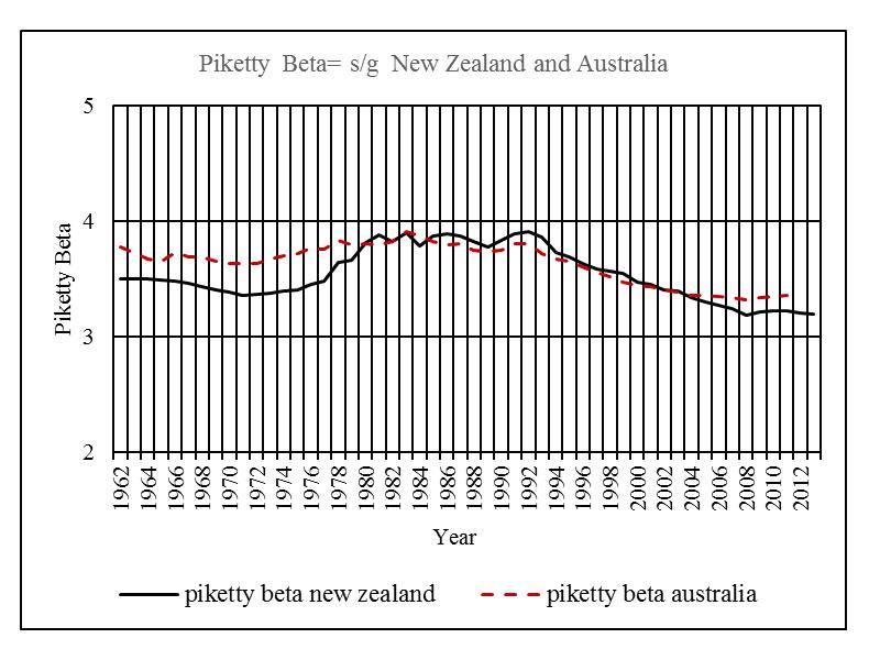
Figure 11 shows inflation for England for the past 700 years.

In England, consumption prices fell by half during the industrial revolution because new technology driven by coal and steam power enabled output to increase faster than the money supply. The elite rentiers (of Jane Austen and Honoré de Balzac fame) referred to throughout Piketty’s book became richer because the value of their inherited fortunes increased relative to incomes. It was sufficient for prices to remain stable or fall with “r” constant leaving their existing wealth intact. That increased the purchasing power in the productive economy leaving the wealthy elite in a better position than they had ever been. Piketty, on the other hand, as demonstrated in Figures 7, 9 and 10 above has produced no evidence to show that (β = s/g) had or has anything to do with that purely monetary process.

The opposite argument applied during the depression years and wartime period when wealth “values” were destroyed first through business and bank collapse, then by wartime destruction and military consumption. As prices rose during wartime, the purchasing power of (some of) the rich declined because government imposed interest rates and capital controls meant that the purchasing power and “wealth” of the rich fell in nominal terms. Rapid inflation increased nominal incomes and saving among workers without the corresponding relative capital growth accruing to the rich. There is nothing magical about that and no “fundamental laws” are needed to explain it. The phenomenon is clear from Figure 10 where “β” in New Zealand increased during the very high inflation – low growth environment rom 1977-1981. It fell again in 1994 and 1995 when growth in New Zealand was the highest it had ever been. Lower inflation following the Basel accords has dramatically reduced measured SNA “saving”. That is what has dominated the change in “β” in recent decades although, as Piketty says, measured economic growth has also been falling as developed economies have become more service-based.

Stabilising “β” is simply a matter of ensuring (s=g), that is, that the money supply (domestic deposits) increases only in line with increased real production. At that point the domestic deposit base increases at the same rate as real GDP and other things being equal:

For stable investment prices inflation must be zero and, using Piketty’s terms, the rate of return “r” on total wealth must then be (r = g/ β)

Figure 11 : CPI (Consumer Price Index) England 1300-2000.

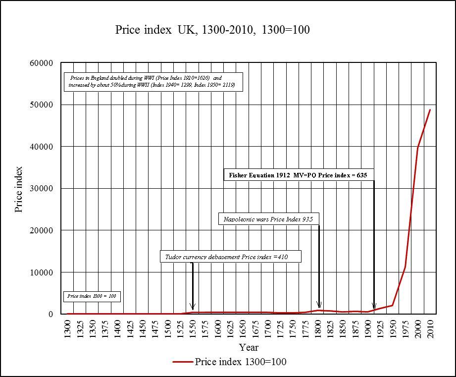
Sources:

Inflation figures 1800-2000: O’Donoghue J, Goulding L (Office for National Statistics Great Britain). Inflation figures 1300-1800 from Gregory Clark “The Price History of English Agriculture, 1209-1914” and Allen G, (House of Commons Library) “Consumer Price Inflation since 1750”, Economic Trends 604, March 2004

6. RECONCILIATION OF GROWTH, SAVING AND INFLATION

The concepts of growth, saving and inflation will now be reconciled with each other.

Nominal GDP growth includes inflation. Production resulting from previous growth costs more each year in nominal terms as inflation increases. Each year after the growth first takes place (and when new assets are created) inflation “revalues” the current monetary worth of that growth. The revaluation is always positive except in recession and depression years.

In Figure 12 the growth figures for New Zealand from 1962-2013 have been reflated backwards, giving a present reflated growth figure of NZ$ 142.8 billion (or 67.5% of current GDP) over the 52 year period. GDP in 1962 was only NZ$ 2.92 billion but the “revaluation” multiplier for 1962 is almost 17, showing that small “original value” amounts of “old” growth have a considerable effect on current GDP. If the “revaluation” exercise were to be taken back further to when the debt-based financial system began, a point which could be called “the beginning of measured growth” would eventually be reached. At that point, the revalued total growth would (for all practical purposes) equal the present GDP.

GDP measures present growth plus all past growth at current prices.

Figure 12. Reflated growth figures New Zealand 1962-2013.

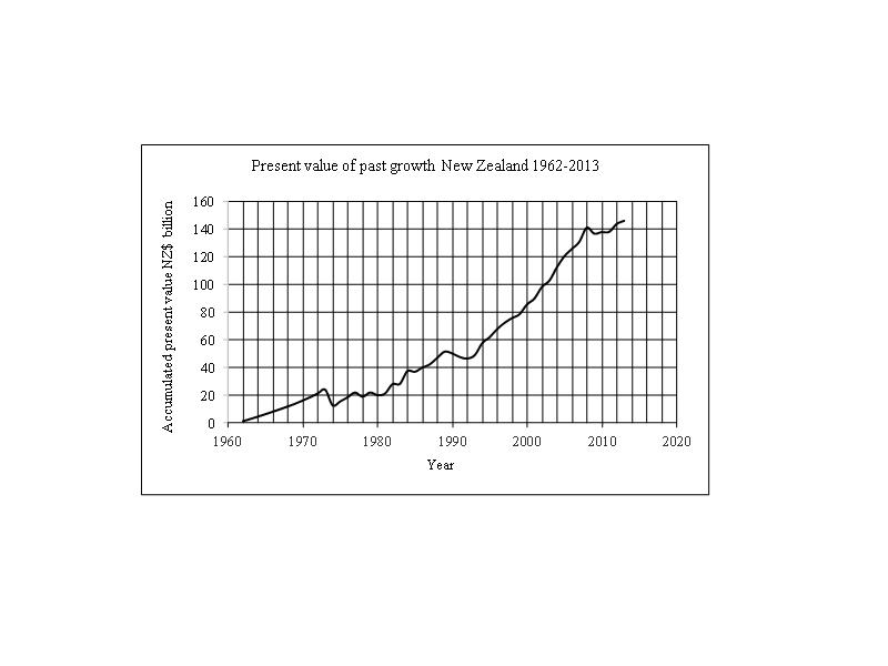
One primary reason there was so very little growth through the middle ages was that there was very little money. Much of what there was was physically hoarded and not invested because there was virtually no inflation and very little to invest in. As Piketty says, until the industrial revolution, most wealth was inherited not earned.

This is because according to the Fisher equation (M*V = P*Q) [see Fisher, I (1912) “Elementary Principles of Economics”] GDP relates to the quantity of goods and services Q the economy produces multiplied by its price P. (GDP = P*Q). “Q” is independent of “P” so that a smaller “Q” means lower GDP unless there is an offsetting rise in “P”. In the Fisher equation “M” is the money supply and “V” is its speed of circulation

While the Fisher equation is typically applied to the productive economy it can equally well be applied to the investment sector in relation to national capital where a subscript “i” is added to the Fisher parameters M,V,P,Q to indicate the investment sector as distinct from the productive economy.

The “value” of national capital is then determined by the available investment sector funding, being the deposit base excluding money needed for physical production of goods and services and its velocity of circulation “Vi” as required by the Fisher equation (PiQi=MiVi), where:

“PiQi” is the traded “output” or investment sector “GDP”, the “value” of national capital exchanged over a given period,

“Mi” is the available investment sector money supply and

“Vi” is the transaction velocity of that investment sector money.

That approach allows the change in net national capital to be calculated at any point in time as long as the asset elements and their respective prices are identified. For example, the cumulative traded “value” of tradable assets “PiQi” might be $100b, “Mi” about $200b and “Vi” about 0.5. If “Mi” increases by 10% while “Vi” remains constant, “MiVi” would increase by 10% to $110b and the national wealth (reflected by market prices) would also increase by 10%.

A similar approach applies to saving too. Nominal GDP appears to be the cumulative sum of past investment measured as the difference between gross capital formation and principal repayments, that is, the outstanding productive sector debt [Manning 2013a, Manning 2012]. In short, production increases with investment in the productive sector. No investment there means little or no monetised production. Even the servants and labourers in pre-industrial times used (expensive) tools and materials when they produced goods and services.

New Zealand GDP was NZ$ 211 billion in 2013 and accumulated SNA “saving”, was NZ$ 169 billion. As previously demonstrated in Figure 5, the difference of NZ$ 42 b between GDP (NZ$ 211 billion) and accumulated saving (NZ$ 169 billion) represents the additional capital repayments physically made over and above the “saving” figures, net of inflation, presently recorded in the national accounts.

The reason productive investment principal is closely related to GDP is conceptually very simple. Tools and equipment wear out and infrastructure and buildings have to be replaced, so that past saving lives on in current capital expenditure (gross capital formation). New investment replaces old investment as recorded by “consumption of fixed capital” in the national accounts. It may be qualitatively different but in principle it produces the “same” amount of output Q. Since the value of new productive assets is included in GDP figures, the value of the increase in new capital stock cannot exceed measured GDP growth. Investment is growth because it generates new production. If that were not so the investment would not be made.

The “missing” 20% or so of GDP (see Figure 5, where a difference of 23% was assumed) referred to above is predominantly due to actual repayments involving amounts over and above the “age and efficiency profile” [depreciation or amortisation] statistics departments use to define the consumption of fixed capital (and therefore the residual “saving” figure “s” ) in the national accounts.

Housing is a problem the world over because once it is constructed it is usually economically unproductive. Servicing the debt and principal repayments on it can only come from productivity increases passed on as higher incomes to income earners or in the form of reduced consumption with all its consequences for growth.

Housing has become unaffordable for an ever increasing number of families because real disposable incomes have not kept pace with real productivity increases (or sometimes even with consumer price inflation) while at the same time inflation has increased asset prices. Moreover, consumption patterns have changed with relatively more disposable income spent on items that were previously “free” or un-monetised, or on transfer payments associated with structural unemployment and welfare caused by economic austerity policies.

The cost of living has changed in ways that the consumer price index CPI fails to include.

The change in affordability is dominated by inflation, that is, by interest rates. One exception in recent times was when US financial institutions distorted the US financial markets by creating bubble debt outside of the productive economy as is also now the case in New Zealand, where the bubble is due in large part to the inward “investment” flows resulting from the country’s current account deficits.

The monetary cost of maintaining the established productive base created by historical investment and growth is very high. Once the investment price of a capital asset at cost has been repaid, (and the initial value of the asset is fully depleted) it is usually replaced. The replacement programme vastly exceeds new productive capital investment which is why the figures in New Zealand’s national accounts for “consumption of fixed capital” are far higher than the figure for Saving. The original investment price is repaid over time in current money at the time of each repayment instalment. The remaining principal repayments on a $1 million investment made 10 years ago, for example, are now being repaid with inflated currency. They are being repaid dollar for dollar irrespective of inflation. However, when the investment is “used up” it takes many more in the meantime inflated current dollars to replace it.

Maintaining a “savings” base to produce the current GDP output in New Zealand presently costs almost 14% of GDP/year so that the average life of the productive assets used to generate the GDP is only about 7 years. That, on the face of it, is a shocking indictment of the waste of any country’s precious national resources.

Cumulative historical savings calculated as outstanding principal on productive capital goods and cumulative historical growth at current prices are both equal to GDP. They are flipsides of the same orthodox economic coin:

(Saving=Investment) (S=I) where the investment is used to pay for the new capital goods the economy produces.

7. WHAT IS CAPITAL?

Table 4.3 “Net capital stock by asset type” found in the New Zealand Statistics Department publication “Measuring Capital Stock in the New Zealand Economy” edition 3, March 2013 indicates there is minimal net financial capital.

In the present debt-based financial system, financial assets are generally offset by counterpart liability. That is due to the double entry bookkeeping of the banking system whereby (domestic credit = deposits + net foreign currency holdings + bank equity + residuals). The secondary debt (on-lending) market follows the same pattern.

This does not mean financial assets in a debt-based financial system are evenly distributed among the population. The opposite is true: broadly speaking the rich have the assets while the poor have the debt.

National accounts only include non-financial, produced, fixed assets. Piketty has not shown how his national account-based factors “r”, “α” , “s”, “g” , that all relate to about half of the national capital, can be extrapolated to form “net national wealth” by way of his single multiplier “β”. Simple ratios such as Piketty’s short term indicators (β= α/r) and ( β = s/g) only confirm that the “value” of wealth is largely a function of inflation because the value of national wealth “β” obviously includes both new and past inflation.

The New Zealand interest rate structure has for decades been among the highest in the developed world. The country also has one of the world’s largest per capita accumulated current account deficits. That means the rate of return “r” on national wealth in other developed countries will typically be lower than the ones shown in Figure 8. By way of contrast, the central bank rate in the world’s biggest developed economies (Europe, US and Japan) is zero for practical purposes so their rate of return “r” on total wealth is likely to be far below 2%. Deposit interest rates are mostly a fraction of one percent while mortgage interest rates in the US are 3% – 4% (fixed for 30 years!), about half those in New Zealand for floating rate debt. Fixed rates in New Zealand are even dearer!

At the same time, unlike New Zealand businesses, US and European businesses typically pay a dividend “yield” of 3% or less. The 2% (or less) rate of return on capital applies to only about half of the total wealth, if New Zealand can be used as an example. The average rate of return on capital in the US, Japan, and Europe is therefore now the region of 1% or less, which is not even remotely like the 5% Piketty talks about in his book [at pp 51-52 for example] despite the notorious tax avoidance by large capitalists and corporations.

In 2013, the present value of the portion of New Zealand’s national capital measured in Table 4.3 of the New Zealand national accounts was NZ$ 620b.

The material presented in this paper suggests that reflating the annual savings in the same way as was done for past growth in Figure 13 gives a present value of produced wealth that can be compared with the NZ$ 620b shown in the national accounts for 2013, assuming the national accounts data is rational.

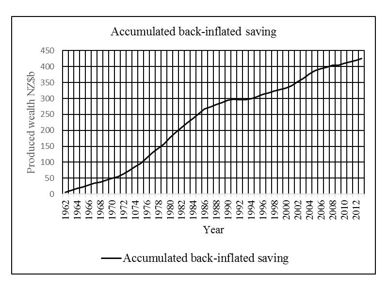
The accumulated saving for New Zealand, as expected, falls well short of NZ$620 billion. The “growth” revaluation for NZ from 1962-2013 shown in Figure 12 accounted for 67.5% of GDP so the best one might have expected is a similar proportion for produced wealth from revalued Saving.

The revaluation exercise for Saving gives a value of produced wealth in New Zealand from 1962-2013 of NZ$ 424.9b or 68.6% of the produced wealth figure shown in the national accounts. That agrees well with the 67.5% of GDP provisionally obtained for accumulated growth over the same period. The proportion would probably remain similar were Saving upgraded to take account of capital repayments as discussed in section 5 because the accumulated growth in Figure 12 would also be higher.

Figure 13. Accumulated back-Saving = Produced Wealth New Zealand 1962-2013.

(lowellpiketty13)

Total produced wealth is the accumulated present value of past Saving.

As a corollary, the “value” of “all wealth” in the absence of bubble debt (section 8) appears to be the present value of past Saving proportionately extended on the basis of supply and demand through market transactions to apply to intangible and non-produced assets.

8. INEQUALITY AND BUBBLES

The previous sections of this paper describe the physical accounting relationships between growth, nominal GDP, saving and wealth.

Using a similar approach to the one already used above for past growth, produced capital (wealth) appears to be the present value of past increases in nominal GDP as set out in section 7 above.

That produced capital is owned by households and businesses that collectively make up the private sector, and the government. In New Zealand (from National Accounts Table 4.3) about half the produced capital (about NZ$ 300b of the total of NZ$ 620b in 2013) is in the form of residential buildings while the rest is non-residential buildings, other construction, transport equipment, plant, machinery and associated equipment and some less tangible assets.

The total net financial wealth owned by households in New Zealand (2013) was about NZ 49b while total net wealth owned by households was about NZ$ 768b (Reserve Bank of New Zealand Table C18). About NZ$ 530b of that household wealth was housing equity, the net value of residential property. That household wealth as well as business wealth is as poorly distributed in New Zealand as it is in the various countries Piketty refers to in his book.

Where there is practically no longer interest paid on deposits, as in the world’s major economies like the US, Japan and much of the EU, inflation is very low and wealth there is expanding slowly if at all. Japan’s GDP, for example, is still expanding despite its slightly declining population, but its domestic credit (money supply) is decreasing. As a result its deposits and measured “wealth” are also decreasing according to the principles set out in this paper.

There is still some inflation in the US (about 1.7% per annum in 2014) but that results from some of the direct monetary stimulus from quantitative easing leaking into the productive economy. The monetary aggregate M3 in US fell by roughly 10% during 2009 due to bankruptcy and business collapse, so the numerical value of national “wealth” would have fallen there by several times that. US asset prices resumed their climb once the wealth destruction bottomed out in 2010. They were higher in 2014 than they were before the 2008 collapse. Physical monetary stimulus outside of the productive economy seems to have produced most of the recent asset price inflation in the US (because annual Saving in the US national accounts is running below 3%). Much of the Quantitative Easing funding is held by financial institutions and does not form part of the M3 money. Its impact on wealth apparently falls outside the national accounts because it is not part of “Saving”.

When deposit interest rates are zero there is no financial transfer from borrowers to deposit holders and therefore no systemic inflation (Manning, 2012). Paying interest to deposit holders means deposit holders literally get something for nothing. That is the biblical definition of usury. The rationale for offering interest on most deposits is twofold: first to protect holders from inflation and secondly to pay deposit holders for “risk” even though there should be little or none in a stable modern banking system. Protecting deposits from inflation through interest rates is a myth because the source papers (Manning 2012, Manning 2013a) show that the interest itself is the cause of systemic inflation. The higher the interest rate, the higher the inflation, as is obvious from a cursory glance at any developed country data set from the time US President Nixon abandoned the US$ gold peg (August 15, 1971) through the resulting 1970’s oil shocks until the Basel I accords were implemented in the late 1980’s. In recent decades, banks have paid competitive interest rates to depositors so as to maintain central bank reserves (liquidity) as required under international banking rules. If they do not pay enough interest their deposits will shift to other banks that pay more. This would create a liquidity crisis because they would not be maintaining enough reserves at the central bank to cover perceived banking risk.

Figure 14 shows how wealth and inequality develop (in the absence of Quantitative Easing provided to financial institutions). The difference between the systemic inflation after tax and CPI inflation shown in Figure 14 seems to be the combined effect of orthodox non-productive saving as described in Section 6.

Figure 14. The source of inequality in New Zealand 1988-2013.

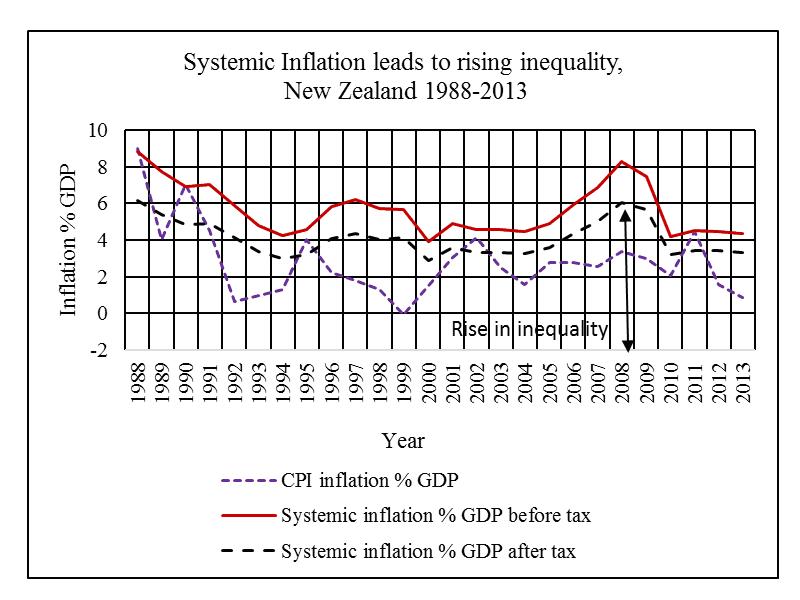
(lowellpiketty14)

Central banks set the floor for interest rates by (arguably, arbitrarily) establishing a base rate at which they will lend fresh liquidity to their participating commercial banks. Raising or lowering that rate effectively controls lending rates to borrowers because, when the price for new money rises, borrowers are unable to borrow as much as they could before, and, overall, new lending falls.

The fundamental issue is that, in aggregate, the borrowers are not the same group as deposit holders. If borrowers already had deposits, they would not typically be borrowing more because it costs much more to borrow than it does to use their existing deposits. Interest rates for borrowing are always higher than deposit rates by an amount equal to the bank spread (the difference between the borrowing or “claims” rate and the “funding” or deposit interest rate).

Inequality increases in proportion to the debt held by an ever-increasing number of poor people relative to the corresponding deposits held by an ever-decreasing number of rich people.

The process of the concentration of deposits in ever fewer hands is gradual. That is why Piketty says inequality has to be viewed over the long term. Just as there is a close association between growth, savings, GDP and “wealth” there is an equally close association in debt –based financial systems between domestic credit (debt), the money supply M3 (excluding inter-institutional lending or “repos”) and GDP. The relationship has become clearer as the influence of cash transactions in generating economic activity has fallen to very low levels in industrialised countries. When cash was “king” some investments could be made from hoarded cash outside the debt-based banking system. That is why from 1900 or earlier until 1990, the ratio (GDP/M3) in New Zealand varied within a narrow range of 1.49 to 1.63 (except for a temporary drop to 1.35 during the depression). Those cash loans produced debt, as has been the case ever since money was invented, but the interest on that debt was personal rather than systemic because the money supply itself was not interest-bearing. Since the late 1980’s, the accumulation of current account deficits and elimination of the cash contribution to economic activity have steadily (almost linearly) reduced the ratio GDP/M3 in New Zealand from 1.63 to 0.82, increasing the money supply as described above and therefore asset inflation.

The increase in MONEY relative to GDP has directly caused asset inflation and that increase is itself caused by deposit interest together with (some) bubble debt.

This gives practical substance to Fulbrook’s profound observations (Fullbrook,2014 p7) That “any increase in the market value of either K [capital] or Y [income] decreases by an equal amount the market value of the other and vice versa …… It is not an accumulation that takes place when capital-2 increases, but rather an appropriation [His emphasis]. While this paper suggests that his “K” would be limited to produced capital, it establishes his notion of transfer or appropriation through saving and inflation from the productive economy by the investment sector.

The two kinds of saving Fullbrook refers to (Fullbrook, 2014 p8) are inflation, his “s_v”, the percent of savings going into existing assets, and growth, his “s_r”, the percent of savings invested in the productive economy.

As an example, consider the monetary figures for New Zealand for 2013 when:

The M1 monetary aggregate was: NZ$ 36.8 billion

M3 excluding repos was: NZ$ 256.1 billion.

The GDP was: NZ$ 211.6 billion

The New Zealand money supply in 2013 was considerably larger than GDP whereas for most of the previous century it was much less than GDP.

Subtracting GDP from M3 left a residual of NZ$ 44.5 billion.

If that residual were reduced by the non-interest-bearing transaction account total M1 (including cash in circulation), which was NZ$36.8 billion in 2013, only NZ$7.7 billion (just 3.6% of GDP) would remain unaccounted for in systemic inflation. That sum unaccounted for represents “bubble” debt, being new debt and its corresponding deposits generated by the banking system outside the productive economy, for example, to pay the outflows resulting from current account deficits when a country is importing too much and living “beyond its means”.

Much (but far from all, in New Zealand’s case) of the current account deficit payments are returned to the debtor country in the form of inward foreign investment flows. To the extent that happens, foreigners literally “buy up” the debtor country as has also been happening in other developed countries like Greece and Spain, as well as New Zealand, not to mention less industrialised countries. The demand by foreigners for debtor country assets determines the currency exchange rates. Some of the inward capital flows are used to invest in productive capacity, but most of them are used to buy existing assets like land and housing. The surplus net inward capital flows increase the domestic deposit base outside of the productive system. Surplus money created to buy a constant quantity of assets is the classic definition of a “bubble” because it inflates existing asset prices over and above the structural effects described in the previous sections of this paper.

The real “bubble” in New Zealand in 2013 was much larger than NZ$ 7.7 billion though, because (as the author sees it) it is by no means true that all of the M1 deposits (in any country) are used for transactions.

Further research is needed to accurately identify the true “bubble” balance but the M1 balance shown in the New Zealand Reserve Bank data for 2013 should probably be reduced by:

a) Most cash in circulation (say NZ$ 3 billion of a total of NZ$ 4b), which is mostly hoarded in the informal economy (in the drug trade and other illegal activities)

b) The deposits used in productive transaction accounts to physically generate GDP that the author estimates at about 5.5% of GDP or NZ$ 11.6 billion

c) The transaction deposits used in the investment sector to physically generate the transfer of existing assets (say 2.5% of GDP or NZ$ 5.3 billion)

The total of (a), (b) and (c) is NZ$ 19.9 billion which is much less than the M1 monetary aggregate of NZ$ 36.8 billion shown in the example above for New Zealand for 2013. The “bubble” debt in the New Zealand example would then increase to NZ$ 44.5 billion less NZ$ 19.9 billion or NZ$ 24.6 billion (11.6% of GDP) instead of the NZ$ 7.7 billion (3.6% of GDP) mentioned above as unaccounted for.

That suggests therefore, bearing in mind the relationships between GDP, savings, and “wealth”, that the entire wealth base in New Zealand was overvalued by roughly 11.6% in 2013.

That is not the end of the story, either, because New Zealand’s net foreign currency assets in March 2013 were NZ$ -47.6 billion. That means there was another NZ$47.6 billion (21% of GDP) that could be invested by foreigners in New Zealand. That did not happen in 2013 because the banks have “arbitraged” the investment flows. They have chosen to keep NZ dollar reserves and instead borrow foreign currency to satisfy their foreign exchange commitments because it has been cheaper for them to borrow abroad (after taking account of the costs of doing so) than it would have been to pay interest on deposits in New Zealand. That leaves New Zealand vulnerable to offshore interests as well as to the banking system, because more deposits returning to New Zealand would create an additional investment “bubble” amounting to a further 21% of GDP, (NZ$ 44.6/211.6 b), in investment prices over and above the 11.6% or so referred to above. New Zealand’s potential “bubble” debt is therefore a whopping 32.6% of its GDP

The reverse applies to surplus countries like Japan, China and Germany who have “exported” (at least some of) their asset inflation to the debtor countries by reducing their deposits relative to their GDP. .

Plainly, in the case of “bubble” deposits, deposit interest accrues to those who sold their domestic assets in return for their bank deposit. From that point on, they miss out on subsequent capital gains from the increase in the price of the asset they have sold, but they retain the capacity to buy another asset, while the deposit remains permanently in the financial system unless or until the corresponding original debt has been repaid. On the other hand, as far as foreign investment goes, the accumulated net foreign asset imbalance can only be rectified by reducing the debtor country’s current account deficits. As long as the current account debt keeps growing, so does the investment “bubble” it has created, leaving the debtor country at constant financial risk.

Over time, the investment sector (taking New Zealand as an example) has expanded beyond the economic growth rate by an amount equal to the inflation represented by the difference between real economic growth on the one hand and (nominal GDP plus the added impact of “bubble” debt as described) on the other.

Since New Zealand has had one of the highest interest rates in the developed world its deposit base has increased rapidly, increasing the amount of deposit interest transferred from borrowers to deposit holders.

The amount of interest transferred from borrowers to subsequent deposit holders from the two sources described above is an accounting identity that can be quantified at any point in time. Its direct result in New Zealand has been a rapid inflation in “wealth” of a small minority of the population and an equally rapid increase in inequality among the population as a whole. Piketty’s data confirms similar trends in other countries too.

That is why so many economists and officials in debtor countries like New Zealand are worried about the “overheating” of the non-productive investment sector, especially housing. They are correct, but the bubble causing the “overheating” is structural, and in the absence of effective measures to correct the imbalances by reducing interest rates toward zero, introducing serious tax reform and reversing the disastrous external deficits, debtor countries like New Zealand are doomed to perpetually increasing inequality and the impoverishment of most of their populations.

Piketty among others observes that unequal wealth distribution is also growing from absurdly high “earned” incomes. While that is true and those “earned” incomes further distort the distribution of wealth and increase inequality, they are not themselves the cause of wealth “generation”. They are a “normal” part of productive sector GDP and their effect on wealth inequality can be addressed by more appropriate progressive taxation .

9. CONCLUSION

Piketty’s “golden rule” and his “laws” do not withstand scrutiny. His own data set for Australia shows his “laws” to be false.

The heart of Piketty’s book and his “laws” is that the percentage (r-g) gives rise to a capital-based unearned income that is surplus to the monetary requirements of the productive economy. That surplus income is created through inflationary deposit expansion that forms part of Saving “s” in the SNA system of national accounts.

Contrary to Piketty’s claims, wealth is transferred upward through the deposit interest rate mechanism whereby the net interest paid by original debt holders under their debt contracts finds it way as unearned income to current deposit holders’ accounts. That unearned income is funded from nominal GDP growth and directly confers higher values on all traded national capital in both the productive economy and the non-productive investment sector.

Inflation coupled with interest rate controls and high taxation caused the “U” shapes in the “β” graphs (national capital/national income) shown in Chapter 3 of Piketty’s book. Neither of his “fundamental laws” explains the historical events he refers to in his book.

After replacing principal repayments for the existing “consumption of fixed economy assets” in the national accounts “SAVING” =NOMINAL GROWTH in the productive sector.

GDP = the sum of existing outstanding productive investment principal.

GDP =the accumulated present value of all past real GDP growth in the productive economy.

Produced capital (wealth) = the accumulated present value of all past saving.

National capital (total wealth as defined by Piketty) = the value of produced capital extended to include produced intangible and non-produced assets. It is determined directly by the size of the domestic deposit base (including deposits resulting from bubbles).

In the absence of bubbles, asset inflation will cease when deposit interest is zero.

In the absence of bubbles (and only then ), using Piketty’s terminology, when deposit interest rates are zero the rate of return “r” on the national capital will be the economic growth rate (g_t/ β). At that point, using Piketty’s typical figures for “β” of 6 and “g” of 2%, “r” would be just 0.33%, not the 5% Piketty refers to throughout his book.

Many developed countries with low interest rates referred to in Piketty’s book may already have a rate of return “r” on national capital of less than 1% because national capital is a function of deposits and saving, not “growth”.

10. REFERENCES

(All the papers by Manning L are published at www.integrateddevelopment.org)

Manning L 2011a,August 2011)“The Interest-Bearing debt System and its Economic Impacts”v. 5 Interest-bearing debt system and its economic impacts. (Revised edition).

Manning L 2011b (September 2011) “The Savings Myth” v. 7

Savings Myth. (Revised edition).

Manning L (October 2012) “The Missing Links Between Growth, Saving, Deposits and GDP” v.3

Missing links between growth, saving, deposits and GDP.

Manning L 2013a (February 2013) “The DNA of the Debt-Based Economy” v.3

DNA of the debt-based economy.

Manning L 2013b (April 2013) “Capital is Debt”

Capital is debt.

Manning L 2013c (September 2013) “The End of Capitalism: Systemic Collapse” v.2

The end of capitalism : Systemic collapse.

Piketty Thomas, “ Capital in the Twenty-First Century” English translation by Arthur Goldhammer, Belknap Press of Harvard University Press, 2014

Piketty Thomas & Zucman Gabriel, “Capital is Back: Wealth-Income Rations in Rich Countries” July 26,2013. piketty@pse.ens.fr zucman@pse.ens.fr

Fulbrook Edward, “Capital and capital: the second most fundamental confusion”, Real World Economics review, issue no 69, pages 149-160, 2014.

A. ORIGINAL PAPERS IN ALPHABETICAL ORDER.

NEW : Beyond Piketty : The Anatomy of Inequality.

Beyond Piketty : The Anatomy of Inequality.

Capital is debt.

Debt bubbles cannot be popped : Business cycles are policy inventions.

DNA of the debt-based economy.

General summary of all papers published.(Revised edition).

How to create stable financial systems in four complementary steps. (Revised edition).

How to introduce an e-money financed virtual minimum wage system in New Zealand. (Revised edition) .

How to introduce a guaranteed minimum income in New Zealand. (Revised edition).

Interest-bearing debt system and its economic impacts. (Revised edition).

Manifesto of 95 principles of the debt-based economy.

The Manning plan for permanent debt reduction in the national economy.

Measuring nothing on the road to nowhere.

Missing links between growth, saving, deposits and GDP.

Savings Myth. (Revised edition).

Unified text of the manifesto of the debt-based economy.

Using a foreign transactions surcharge (FTS) to manage the exchange rate.

(The following items have not been revised. They show the historic development of the work. )

Financial system mechanics explained for the first time. “The Ripple Starts Here.”

Short summary of the paper The Ripple Starts Here.

Financial system mechanics: Power-point presentation.

B. REVIEWS.

Analysis of Jackson, A., Dyson, B., Hodgson, G. The Positive Money Proposal – Plan for Monetary Reform, Positive Money, London, 02 April, 2013. (Posted 11 May, 2013.)

Analysis of the New Zealand Initiative (NZI) paper by B. Wilkinson : New Zealand’s Global Links : Foreign Ownership and the Status of New Zealand’s Net International Investment. (Posted 11 May, 2013.)

Chicago Plan Revisited Version II: An insufficient response to financial system failure. (Posted 11 May, 2013.)

Comments on the original IMF (Benes and Kumhof) paper “The Chicago Plan Revisited”. (Posted 20 August, 2012.)

C. ARTICLES.

The end of capitalism : Systemic collapse. (24 August, 2013).

Increases in export income from price rises abroad are not growth. (26 August, 2013).

There’s no such thing as affordable housing. (15 June, 2013).

What about a tax cut for the poor? (16 May, 2013).

D. OTHER.

Carroll, W.K.; Sapinksi, J.P., The Global Corporate Elite and the Transnational Policy-Planning Network, 1996-2006 : A Structural Analysis, International Sociology, Vol. 25 no. 4 pp. 501-538, Sage Publications, Thousand Oaks, July 2010.

Vitali S. et al, The network of global corporate control. Swiss Federal Institute of Technology (ETH), Zurich, October, 2011.

The Transnational Insitute (TNI), Amsterdam, 2013 : State of Power : Dirty Money : The finance and fossil fuel web. “Banks and fossil fuel companies not only make up the wealthiest corporations, they sit on each others boards and their executives include some of the world’s most powerful political and social institutions.”

For the domination of the financial lobby in European decision making see Wolff, M. and others, The Fire Power of the Financial Lobby : A Survey of the Size of the Financial Lobby at EU Level, Corporate European Observatory (CEO) with the Austrian Federal Chamber of Labour and the Austrian Trade Union Federation IÖGB), Brussels, April 2014. Understating reality by using minimal salaries and excluding event organisation, travel costs and taxation, some 1700 financial lobbyists working for 700 organisations (450 of which are unregistered) spend € 123 million a year on lobbying EU institutions, 30 times more than NGOs, Trade Unions and Consumer Associations together. They account for more than 70% of lobby meetings with EU institutions and have dominated with up to a 94% participation 15 out of the 17 “Expert Groups” on financial topics, the exceptions being the two “users” groups.

Super-secret negotiations are under way which would still further expand the almost unlimited dominating power of the finance industry. See Wikileaks Secret Trade in Services Agreement, under negotiation, Annex 10. For preliminary comments on it see Kelsey J, Memorandum on the Leaked [Secret] TISA [Trade in Services] Financial Services Text which is also published by Wikileaks.

By every measure, the big banks are [37%] bigger [than in 2008], S.Gandel, fortune.com, Time Inc, 13 September, 2013.

---

This work is licensed under a Creative Commons Attribution-Non-commercial-Share Alike 3.0 Licence..